

Theory of Consumer Demand
The theory of consumer demand explains how consumers make choices about what goods and services to purchase and how much to spend, given their preferences, income, and prices. This theory helps us understand how consumers allocate their limited resources to maximize their satisfaction or utility.
Important components and concepts of theory of consumer behavior are utility, preferences, budget constraint, consumer equilibrium and demand carve. The theory of consumer behavior is based on the axiom that individual is a utility maximizing entity i.e. individual tries to maximize the benefit it gains from consuming the goods and services given their budget constraint.
Utility
Utility is a core concept in economics which helps understand how individuals make choices. When a consumer buys or demands a particular commodity he derives some benefit from its use. He feels that his given want or need is satisfied by the use or consumption of the commodity purchased. This want satisfying power of a commodity is called utility.
The concept of ‘utility’ was introduced to social thoughts by Jerenmy Bentham in 1789 and to economic thoughts by Jevons in 1871 In economic sense, Utility is a psychological phenomenon that refers to the feeling of satisfaction, pleasure, happiness or well-being a consumer derives from the consumption or possession of a commodity. Utility can also be defined as the power or ability of a good or service to satisfy a human want or need.
Kinds of Utility
- Total Utility (TU) is the total satisfaction derived from consuming all the units of a good or service. In other words, it is the sum of marginal utilities.
- For example, if an individual consumes n units of a single commodity, then

- Marginal Utility (MU) is the additional satisfaction that an individual derives from consuming an additional unit of a good or service. Thus, MU is the change in total utility obtained from consuming one additional unit of a commodity. MU=∆TU/∆Q. MU may also be expressed as

- Average utility (AU) is the total utility divided by number of units consumed. For example, if TU by consuming 4 units of a commodity is 40 utils then AU will be 10 utils.


Relationship Between Total Utility and Marginal utility
MU can be either positive, zero or negative. Positive MU occurs where consumption of an additional unit of commodity makes addition to TU. Zero MU occurs where consumption of additional unit does not add to TU, this is called satiation point and Negative MU occurs where consumption of additional unit decreases TU and cause dis-satisfaction.
Table 1: Relationship Between Total Utility and Marginal utility
| Total Utility | Marginal Utility |
| When TU increases at decreasing rate | MU decreases and but remains positive |
| When TU decreases | MU becomes negative |
| When TU is maximum | MU is zero |
Characteristics of Utility
- Utility has no ethical or moral significance
- Utility is psychological; depends on mental attitude
- Utility is relative; varies in different situations
- Utility is different from usefulness
- Utility depends on the intensity of want
- Utility is different from pleasure
Approaches to Measure Utility
Now the question arises how to measure utility? Different schools of thought differ on the measurability of utility. The Classical and Neoclassical economists assume that ‘utility is measurable cardinally’, i.e., measurable in terms of cardinal numbers (1, 2, 3 and so on).
The modern economists believe that ‘utility is measurable only ordinally’, i.e., in terms of preferability of one good over another. This has lead to two main approaches to the analysis of consumer demand, 1. Cardinal utility approach and 2. Ordinal utility approach.
Cardinal Utility Theory
Introduction to Cardinal Theory
Cardinal utility analysis is the oldest theory of demand which provides an explanation of consumer’s demand for a product and derives the law of demand. The cardinal utility approach assumes that utility is measured in cardinal numbers Cardinal utility approach also known as Marshallian approach explains consumer behavior with two laws:
- The Law of Diminishing Marginal Utility (Gossen’s First Law)
- The Law of Equi-Marginal Utility (Gossen’s Second Law)
Utility refers to the satisfaction or pleasure that consumers receive from consuming a good or service. Marginal utility is the additional satisfaction that is received from consuming an additional unit of a good or service.
Assumptions of Cardinal Utility Approach
Cardinal Measurement of Utility: Utility is a measurable and quantifiable entity. According to Marshall, utility is actually measurable in terms of money. He argues that the amount of money which a person is willing to pay for a unit of a good is a measure of utility.
Some economists belonging to the Cardinal school measure utility in imaginary units called “utils”. For example, if a thirsty person is willing to pay Rs 50 for one can of Pepsi, his/her utility of one can of Pepsi is 50 utils.
Utility is Independent: Utility which a consumer obtains from one good say X is the function of quantity of that good X only, it does not depend upon the quantity consumed of other goods say Y. Thus, U_X=f(Q_X). This assumption states that utility is ‘additive’, that is, separate utilities of different goods can be added to obtain the total utility. Thus, TU=TUA+TUB.
Constant MU of Money: Utility that the individual derives from spending money on various goods is assumed to be constant. Measurement of marginal utility of goods in terms of money is only possible if the marginal utility of money itself remains constant.
Consider a case when price of a good falls which raises the real income of the consumer the marginal utility of money to him will fall and the consumer will decrease the demand for goods, but Marshall ignored this and assumed that marginal utility of money did not change as a result of the change in price.
Rationality: It means that consumer aims to maximize his/her utility therefore, he first buys a commodity which yields the highest utility, and he buys last a commodity which gives the least utility.
Diminishing MU: Utility obtained from consuming each additional unit of a commodity goes on to decrease.
Money Income and prices are given: The consumer has a fixed limited money income to spend on the goods and services he chooses. Moreover, he has no influence to changes prices.
Law of Diminishing Marginal Utility (DMU)
Introduction to Law of DMU
“The Law of Diminishing Marginal Utility states that as a consumer takes more units of a good, then extra utility derives from an extra unit of the good goes on falling”. In other words, marginal utility of a good diminishes as an individual consumes more units of a good. Thus, the law of diminishing marginal utility means that the total utility increases at a decreasing rate.
This law is based on the fact that total wants of a man are virtually unlimited, but each single want is satiable. Therefore, as an individual consumes more and more units of a good, intensity of his want for the good goes on falling and a point is reached where the individual no longer wants any more units of the good, this is called saturation point. It is defined as: The point at which TU is at its maximum and MU is zero is known as the saturation point.
Graphical Illustration of the Law of Diminishing MU
The law of diminishing Marginal utility can be explained with the help of a schedule and graph. In figure 1 we measure units of good X (sandwich) on horizontal axis and TU of good X (sandwich) on vertical axis. We can see that as we consume more units of good X TU increases at a decreasing rate upto the 5th unit, TU is maximum at 5th unit and then TU decreases. When TU is increasing MU remains positive, when TU is maximum MU is zero, this is called satiation point. After satiation point TU decreases and MU becomes negative.
Table 1: Total Utility Schedule
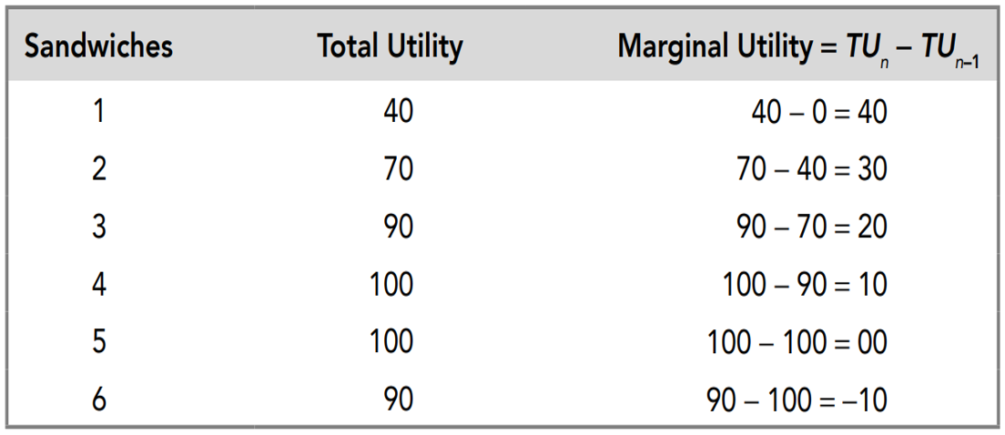
Figure 1: Total Utility Curve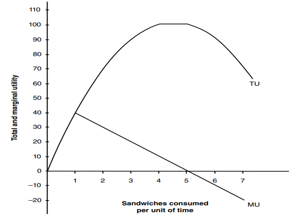
Assumptions of the Law of DMU
The law of diminishing MU holds only under certain given conditions. These conditions are often referred to as the assumptions of the law.
- First, the unit of the consumer goods must be standard. If the units are small or large, the law may not apply.
- Secondly, consumer’s taste and preference remains unchanged during the period of consumption.
- Thirdly, there must be continuity in consumption.
- Fourthly, the mental condition of the consumer remains normal during the period of consumption.
Mathematical form of Utility Function
The law of diminishing MU suggests the following quadratic utility function.  . Suppose a specific utility function for sandwich
Interpretation:
- Initial Utility: The linear term 45X shows that utility initially increases with the consumption of sandwiches.
- Diminishing Marginal Utility: The negative quadratic term
 indicates that as the quantity of sandwiches consumed increases, the additional utility gained from consuming each additional sandwich decreases.
 indicates that as the quantity of sandwiches consumed increases, the additional utility gained from consuming each additional sandwich decreases.
Consumer Equilibrium: A Single Commodity Case
A consumer consumes several commodities and attains his equilibrium when he maximizes his TU given his income, and prices of commodities he consumes. First, we consider the case of single commodity say X. because money and commodity X both provide utility to the consumer.
The additional utility a consumer gains from consuming additional unit of commodity X is called MU of X. Further assume that consumer purchase one unit of commodity X at price Px. A consumer can either spend the money or can retain it with himself. If he retains all the money, then MU of money is very low which is less than MU of acquiring first unit of commodity X.
The consumer can increase its utility by consuming commodity X. Due to law of diminishing MU an increase in consumption of X reduces MU of X. He consumes commodity X as long as  . Because MU of money is 1, thus consumer will be in equilibrium if
  .
.
Explanation through Diagram of Consumer Equilibrium
Figure 2: Consumer Equilibrium: Single Commodity Case
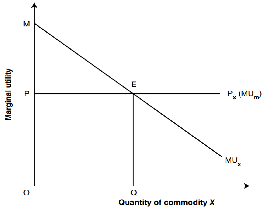
The horizontal line Px.(MUm) shows the constant utility of money weighted by Px (the price of commodity X) and MUx curve represents the diminishing MU of commodity X. The Px (MUm) line and MUx curve intersect at point E, where MUx = Px (MUx ). Therefore, consumer is in equilibrium at point E.
At any point above E, MUx > Px (MUm). Therefore, if a consumer exchanges his money income for commodity X, he increases his satisfaction per unity of commodity. At any point below E, MUx < Px (MUm), the consumer can therefore increase his satisfaction by reducing his consumption of commodity X. Therefore, point E is the point of consumer’s equilibrium.
A Numerical Example
Suppose a consumer has USD 100 and is deciding how much of a single good (say apples) to buy. The price of one apple is USD 2; the marginal utility of money (MUm) is 5 utils. Spending USD 2 on an apple gives up 𝑃*(𝑀𝑈𝑚)=2*5=10 utils of satisfaction from money.
- The consumer will buy apples until 𝑀𝑈x=𝑃⋅(𝑀𝑈𝑚)=10.
- 1st apple: 𝑀𝑈x=14>10, so the consumer buys it.
- 2nd apple: 𝑀𝑈x=11>10, so the consumer buys it.
- 3rd apple: 𝑀𝑈x=8<10, so the consumer does NOT buy it.
Equilibrium is achieved at 2 apples, where 𝑀𝑈𝑐=11, which is still slightly above 𝑃⋅𝑀𝑈𝑚, but buying another apple would result in 𝑀𝑈x<𝑃⋅(𝑀𝑈𝑚).
Derivation of Demand Curve through Law of DMU
The basic purpose of the analysis of consumer behaviour is to derive a consumer demand curve. Marshall3 was the first economist to explicitly derive the demand curve from consumer’s equilibrium condition for a single commodity, say X, as MUx = Px.
Diagram
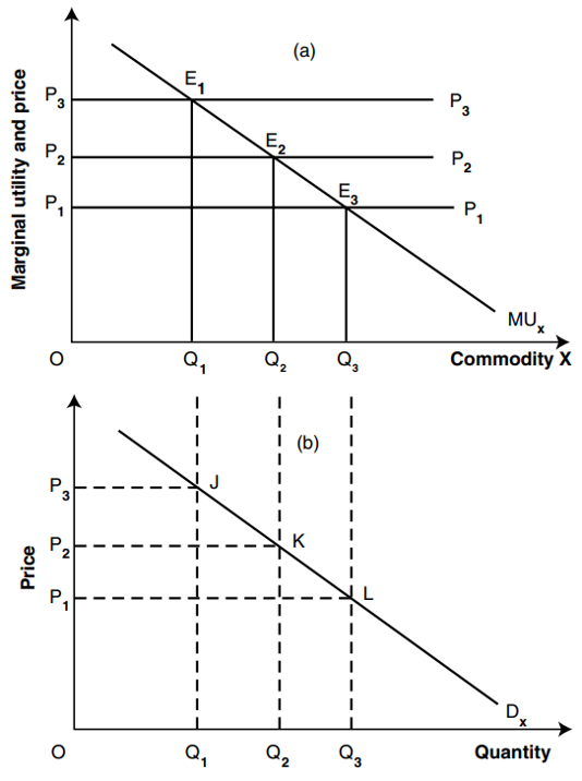
Figure 3: Derivation of Demand Curve through Law of DMU
Explanation
The upper panel of figure shows MUx and Px and lower panel shows the relationship between Px and quantity consumed or demanded of commodity X. Consumer is initially in equilibrium at E1 where MUx=P3 and he consumes Q1 units (upper panel). Therefore, at P3 quantity demand is Q1 units (lower panel). As price falls to P2 the equilibrium condition disturbs and MUx>P2. He can increase his TU by spending on good X and Mux falls again to P2 where consumer demands Q2 quantity.
Thus, at P2 quantity demanded is Q2. Similarly, at P1 quantity demanded is Q3. This gives us the relationship between price of X and quantity demanded of good X. When price of X is lower consumer demands higher quantity of X so as to equate Mux with Px. Thus, due to the law of diminishig marginal utility demand curve has negative slope.
Applications and Uses of Law of DMU
Firstly, we can derive demand curve from the law of DMU. It is due to the law of diminishing marginal utility that the demand curve has negative slope. When price of a good X falls the MUx becomes greater than Px, it disturbs the equilibrium condition. For equilibrium Mux must fall, this can only be happened if we consume more units of X. Thus, to balance the Mux with Px consumer increases demand for good X.
Secondly, the concept of MU help us to explain the paradox of value. According to the modern economists’ price of a good is determined by MU of a commodity. Water which is in abundant quantity has lower MU therefore it has low value in exchange (low price). But diamonds which are scarce relative to water has MU quite high therefore diamonds has high price.
Thirdly, law of DMU helps government in the redistribution of income which increases overall welfare. Just as law of DMU applies on commodity, this law also applies on money. Govt. impose taxes on rich and transfer this income to the poor i.e. Govt. takes utility from the rich and transfer this utility to the poor.
It is obvious that utility gain of poor is greater than utility loss of the rich. Because for rich person MU of money is less so he loses less and MU of money for poor is high, so he gains more. Thus, it increases total welfare of the society.
Fourthly, the Marshallian concept of consumer’s surplus is also based upon the principle of diminishing marginal utility.
Law of Equi-Marginal Utility
Law of Equi-Marginal Utility is also known as Gossen’s Second Law or law of substitution or law of maximum satisfaction. Suppose there are only two goods X and Y on which a consumer has to spend a given income. When consumer spend his money income he has two things in mind, marginal utilities associate with goods X and Y and prices of both goods.
Law of Equi-Marginal Utility states that “the consumer will distribute his money income between the goods in such a way that the utility derived from the last rupee spent on each good is equal.” In other words, consumer is in equilibrium position when marginal utility of money expenditure on each good is the same. Now, the marginal utility of money expenditure (MUe) on a good is equal to the marginal utility of a good (MUx) divided by the price (Px) of the good.

Suppose that consumer distributes his income on two goods X and Y. The equilibrium condition for both goods is:


By including the marginal utility of money to this equilibrium condition:

Thus, the consumer will be in equilibrium when the above equation holds. If the consumer consumes n goods, then;

Graphical Illustration of Law of Equi-Marginal Utility
| Units | MUx | MUy | MUx/Px | MUy/Py |
| 1 | 20 | 24 | 10 | 8 |
| 2 | 18 | 21 | 9 | 7 |
| 3 | 16 | 18 | 8 | 6 |
| 4 | 14 | 15 | 7 | 5 |
| 5 | 12 | 12 | 6 | 4 |
| 6 | 10 | 9 | 5 | 3 |
Diagram
Figure 4: Law of Equi Marginal Utility
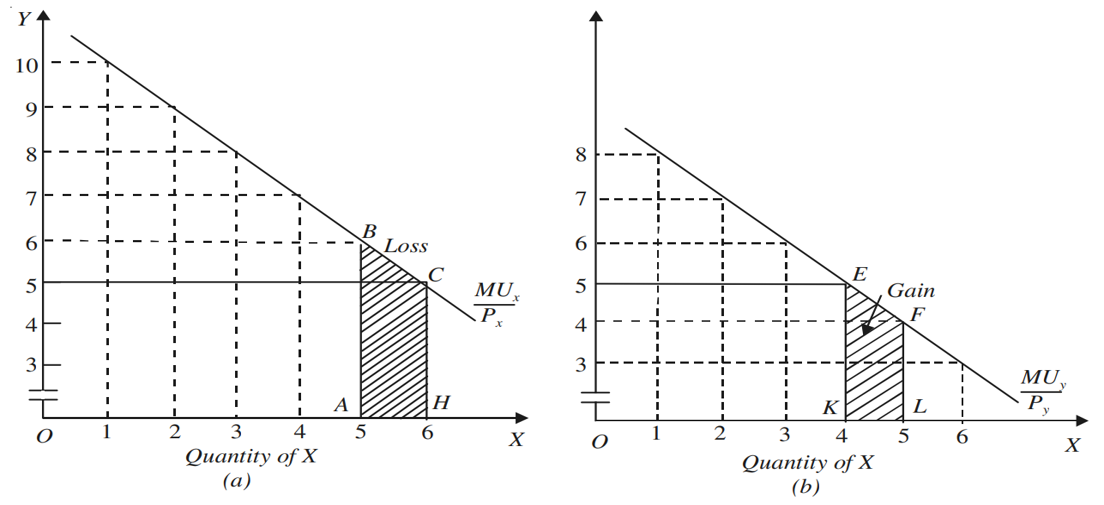
Suppose that consumer spend his money income of Rs. 24 on two goods X and Y given their prices Rs. 2 and Rs. 3 respectively. To get MU of money expenditure we divide MUx with 2 and MUy with 3.
Now the consumer will equate the marginal utility of the last rupee (i.e. marginal utility of money expenditure) spent on these two goods. This happens when he consumes 6 units of good X and 4 units of good Y.
Therefore, consumer will be in equilibrium when he is buying 6 units of good X and 4 units of good Y and will be spending (Rs. 2 × 6 + Rs. 3 × 4 ) = Rs. 24 on them.

No other allocation of money expenditure will yield greater utility than when he is buying 6 units of commodity X and 4 units of commodity.
Suppose if the consumer buys 5 units of good X and 5 units of good Y. This will lead to the decrease in his total utility. This can be seen from figure 4. The loss of utility from consuming 5 units instead of 6 is equal to shaded area ABCH and utility gain from consuming 5 units of good Y instead of 4 is equal to shaded area KEFL which is less than ABCH, thus total satisfaction will fall by reallocating his budget.
Limitations of the Law of Equi-Marginal Utility
Consumers are not always rational: The law assumes that consumers rationally calculate and compare marginal utilities of different goods to maximize satisfaction. However, in real life, consumers are often influenced by habits and customs rather than rational calculations.
Cardinal Measurement of Utility: For the law to work, marginal utilities must be measured in cardinal terms (specific units). However, utility, being a subjective feeling, cannot be objectively measured. This limitation has led to the use of ordinal utility analysis, like indifference curves.
Indivisibility of Goods: The law struggles with indivisible goods, like cars, which cannot be purchased in small units. This makes it impossible to equate the marginal utility of money spent on such goods with divisible goods like foodgrains, creating barriers to equalizing marginal utilities.
Suggestions for further reading:
