Population Regression Function and Sample Regression Function

In the previous post we explained the concept of regression analysis in detail along with its meaning, uses and objectives. Moreover, we also discussed how regression analysis differs from correlation analysis and causation. Further, we differentiate conditional and unconditional mean. To read previous article click Nature of Regression Analysis. In this post we will go beyond and discuss the concepts of population regression function and sample regression function with a concrete example. So, let’s start our journey from defining population and sample.

Table of Contents

Population

Population refers to the entire group of individuals or entities about which inference is to be made. For example, if a researcher wants to study the average consumption and income of all households in a city the population will consist of every household in that city.

Sample

Sample is a subset of population that is selected to represent entire population. For example, a researcher, rather than collecting consumption and income data on all households in a city, he randomly selects some households to make an inference about the average consumption and income of all households.

Population Regression Function (PRF)

Population regression function or conditional expected function shows the functional relationship between conditional mean value of dependent variable Yi given the values of independent variable, Xi.

$E(Y_i \mid X) = f(X_i)$

$E(Y \mid X_i) = \beta_0 + \beta_1 X_i$

where β₁ and β₂ are unknown but fixed population parameters known as the regression coefficients; β₁ and β₂ are also known as population intercept and population slope coefficients, respectively.

An Example

To clear the meaning of regression let’s consider an example where we want to study the relationship between consumption expenditure and disposable income of 60 families (entire population). The data is given in table 1 and is taken from the book of Gujarati, Basic Econometrics 5e, table 2.1.

Table 1: Data on consumption and income of 60 families (population)

Y ↓ / X →	80	100	120	140	160	180	200	220	240	260
Weekly family consumption expenditure Y, $	55	65	79	80	102	110	120	135	137	150
	60	70	84	93	107	115	136	137	145	152
	65	74	90	95	110	120	140	140	155	175
	70	80	94	103	116	130	144	152	165	178
	75	85	98	108	118	135	145	157	175	180
	–	88	–	113	125	140	–	160	189	185
	–	–	–	115	–	–	–	162	–	191
Total	325	462	445	707	678	750	685	1043	966	1211
Conditional means of Y, E(Y\|X)	65	77	89	101	113	125	137	149	161	173

Data in table 1 represents the whole population where Y is weekly consumption expenditure and X weekly income. Economic theory suggests that consumption expenditure increases with the increase in income. Regression analysis predicts the mean consumption on the basis of various values of independent variable.

From the table we can see that there is considerable variation in weekly consumption expenditure in each income group. For example, all households with weekly income of USD 80 have weekly consumption ranges from USD 55 to USD 75, similarly households with weekly income USD 100 have weekly consumption ranges from USD 65 to USD 88. Moreover, there are also considerable variations in consumption across all other groups.

Note that on average, weekly consumption expenditure increases as income increases (see last row). In other words, households with higher level of income have higher consumption levels and households with lower income levels have lower consumption expenditure. For example, average weekly consumption of households whose income is USD 80 is USD 65, and average weekly consumption of households whose income is USD 160 is USD 113. Note that we are not talking about consumption of each individual family and their income rather we are talking about mean consumption of each income group.

Population Regression Line (PRL)

Figure 1: Population regression line

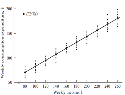
Population regression line or population regression curve is the locus of conditional means values of dependent variable Y, for each fixed or given values of independent variable. More simply, it is the curve connecting the means of the sub populations of Y corresponding to the given values of the regressor X.

The population regression line in Figure 1 connects the conditional means of consumption (dark dots) at different income levels, represented by circles showing average consumption values for each income level. At any given income, such as USD 80, consumption can vary within its probability distribution, indicating that not all households with the same income will have identical consumption expenditures; rather, their average could be USD 65. Regression analysis aims to estimate this average consumption at various income levels, rather than predicting individual household consumption.

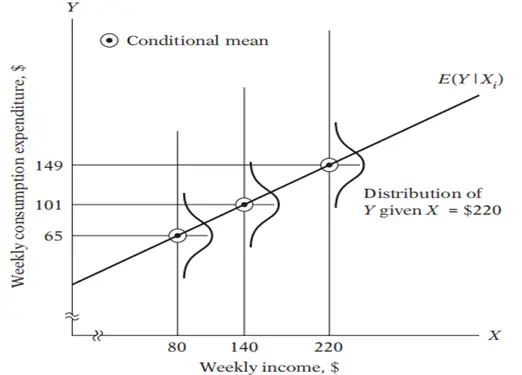
Figure 2: Conditional means of Y

Stochastic Specification of PRF

So far, we see situation where we study the relationship between mean consumption and income. In figure 1 when we draw their graph all points lie on the same upward sloping line (see dark dots that represent mean consumption at each income level). This is an example of a mathematical model. But what about consumption of individual family consumption? In figure 1 we see that corresponding to each income level the consumption of each family is clustered around the mean consumption. It means that consumption varies within each income group.

For example, households with income level of USD 80, their consumption varies between USD 55 to USD 75. Which factor causes their consumption to vary although they have same income level? These are the factors other than income that are responsible for this variation. It might be happened that two families may have same income level (say USD 80), but their consumption does not the same due to the difference of family size. A family with more members naturally has more consumption.

The model accounts for family size but still leaves unexplained variation not accounted for by income and family size, due to unmeasurable factors and potential measurement errors, such as inaccurate income reporting. Regression analysis aims to estimate average consumption behavior across families rather than individual consumption, necessitating the inclusion of a random error term to represent omitted factors affecting the outcome.

Thus, due to these factors each family consumption may differ from average consumption. The difference between each family`s consumption and conditional mean family consumption is called stochastic error term. When we introduce stochastic error term in PRF we get stochastic PRF. It can be written as:

$u_i = Y_i - E(Y \mid X_i)$

$Y_i = E(Y \mid X_i) + u_i$

Substituting the value of E(Y | X_i) in last equation which is β₀ + β₁ X_ifrom eq 2.

$Y_i = \beta_0 + \beta_1 X_i + u_i$

Remember that an econometric model is a set of behavioral equations which has some observed variables, and some unobserved variables. The observed variables are those that are included in the model also called independent variables which explain the variations in Y, the dependent variable. For example, in our consumption function example consumption is a dependent variable whose variation we try to explain, and income is an independent variable who explains the variation in consumption.

There is not only one factor that affects consumption. There are lot of unobserved factors that can afect consumption, but these factors are not explicitly included in the model. The effect of these omitted factors is capture by the disturbance term. Thus, we can say that consumption of each family is the sum of mean consumption of all families at a particular income level pus a random error term. The stochastic error term captures the effect of all those omitted variables that are not explicitly included in a model but collectively affect the dependent variable, Y.

Sampe Regression Function (SRF)

Study of whole population is difficult as it is time consuming, energy consuming, and resource consuming. That`s why we instead of studying whole population we take a sample of this population which is the representative of whole population. Thus, in regression our task is to estimate the population regression function on the basis of sample regression function. In fact, we can draw “N” number of random samples, and each random sample is not likely to be the same.

The Sample Regression Function (SRF) is the estimated regression equation obtained from a sample of data. It is used to predict the value of the dependent variable given specific values of the independent variables. The linear SRF can be written as:

$\hat{Y}_i = \hat{\beta}_0 + \hat{\beta}_1 X_i$

In PRF our purpose is to find the average weekly consumption on the basis of given or fixed values of income. In SRF our task is to predict or estimate PRF. Remember that we cannot accurately forecast PRF using SRF because of sampling fluctuations. Because we can draw “N” samples from a given population there will be “N” SRFs. Each SRF will provide a different estimate of population parameters.

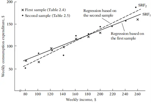
Suppose that we took two random samples from a population of 60 families as given in table 2 and draw sample regression line for each sample SRL₁and SRL₂. Which SRL is true representative of PRL. There is no way we can be absolutely sure that either of the regression lines shown in Figure 3 represents the true population regression line due to the sampling fluctuations.

Table 2: Random samples of 60 families

Sample 1		Sample 2
Y	X	Y	X
70	80	55	80
65	100	88	100
90	120	90	120
95	140	80	140
110	160	118	160
115	180	120	180
120	200	145	200
140	220	135	220
155	240	145	240
150	260	175	260

Sample Regression Line

The sample regression line is the graphical representation of the sample regression function. It is a line that best fits the scatter plot of the observed data points. The line minimizes the sum of the squared differences between the actual values and the predicted values.

Figure 3: Sample regression lines

Sample regression line in linear form can be written as:

$\hat{Y}_i = \hat{\beta}_0 + \hat{\beta}_1 X_i$

We can also write our SRF in another form.

${Y}_i = \hat{\beta}_0 + \hat{\beta}_1 X_i + \hat{u}_i$

Estimator and Estimate

An estimator is a rule or formula or method that tells us how to estimate the population parameter from the sample information. A particular numerical value obtained by the estimator is called estimate. Estimator is random whereas estimate is nonrandom.

Error vs Residual

Error is the difference between the actual value of Y in the population and the conditional mean of Y denoted as E (Y |X_i) in the entire population.

$u_i = Y_i - E(Y \mid X_i)$

Residual is the difference between the actual observed value of the dependent variable (Y) and the estimated value of Y, $\hat{Y}_i$ obtained from the sample regression function (SRF). Residuals are calculated using the data from the sample and represent the deviations of actual values from the fitted regression line.

Looking Forward…

To sum up, then, we find our primary objective in regression analysis is to estimate the PRF

$Y_i = \beta_0 + \beta_1 X_i + u_i$

on the basis of the SRF

${ Y}_i = \hat{\beta}_0 + \hat{\beta}_1 X_i + \hat{u}_i$

We know that we can have as many SRF as number of random samples, so our question is which SRF best approximate the PRF. But in practice neither we have population data to estimate PRF nor we have repeated samples, therefore we have only one SRF in practice and that SRF we obtain from sample data is just an approximation of true PRF.

Figure 4: Sample and population regression lines

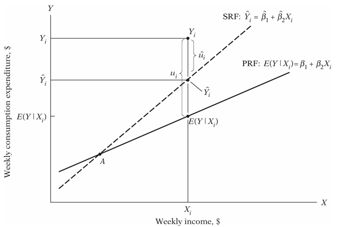
Consider figure 4 where we draw both sample and population regression functions together. We can see that estimated value of, $\hat{Y}_i$ at X=X_i and Y=Y_i, overestimates the E(Y | Xi) for the Xi. An any value Xi to the left of point A, SRF underestimates PRF. But this over and under estimation is inevitable due to sampling fluctuations. So, our purpose is to find the best approximation of PRF.

Can we devise a rule or a method that will make this approximation as “close” as possible? In other words, how should the SRF be constructed so that $\hat{\beta}_0$ is as “close” as possible to the true $\beta_0$ and $\hat{\beta}_1$ is as “close” as possible to the true $\beta_1$ even though we will never know the true β₀ and β₁? The answer is YES, and this method is called Ordinary Least Square Method which minimizes the sum of squared residuals. Sum of squared residuals is equal to sum of squared difference between actual value of Y and estimated value of Y, that is $\sum_{i=1}^{n} \hat{u}_i^2$ or $\sum_{i=1}^{n} (Y_i - \hat{Y}_i)^2$ or $\sum_{i=1}^{n} (Y_i - \hat{\beta}_0 - \hat{\beta}_1 X_i)^2$ .

Suggestions for further readings

Estimating the Population with the Sample Regression Function • Economics.Town

Share this article

Muhammad Minhaj Akhtar

Muhammad Minhaj Akhtar is a Lecturer in Economics at Government Graduate College Jauharabad, Pakistan. He holds an M.Phil. in Economics from Quaid-i-Azam University, Islamabad, and an MSc in Economics from the University of Sargodha, where he earned a Silver Medal. His academic passion lies in Econometrics, with a strong focus on applying empirical methods to real-world economic issues. Through MinhajMetrixHub, he shares learning resources, research guidance, and practical econometric insights for students and researchers.

Read Posts

One Response

Pingback: Simple Linear Regression Model - MinhajMetricsHub

Population Regression Function and Sample Regression Function

Population

Sample

Population Regression Function (PRF)

An Example

Population Regression Line (PRL)

Stochastic Specification of PRF

Sampe Regression Function (SRF)

Sample Regression Line

Estimator and Estimate

Error vs Residual

Share this article

Muhammad Minhaj Akhtar

One Response

Leave a Reply Cancel reply

CATEGORIES

TAGS

Recent Posts

Microeconomic Household Fertility Theory

Inflation, Its Types, Causes and Effects

Malthus Population Theory

Nominal GDP, Real GDP & GDP Deflator

Solow Model of Economic Growth