
In the previous couple of blogs, we discussed the Lewis Theory of Economic Development and International Dependence Model. In this blog our focus is on neoclassical long run economic growth model.
Introduction of Solow Model of Economic Growth
The Solow model of economic growth is a well-known Neoclassical exogenous growth model presented by Robert Solow in an article “A contribution to theory of economic growth” in 1956. This model explains that long-term economic growth depends on three factors:
- Rate of capital accumulation (K)
- Labor force growth
- Technological progress
This model is an extension of Harrod-Domar growth model. Prof. Solow assumed that Harrod-Domar’s model was based on some unrealistic assumptions like fixed factor proportions and constant capital output ratio etc.
The Solow Growth Model implies that all countries will have same level of income if they have same rate of saving, labor force, depreciation and productivity growth, this is known as conditional convergence.
Assumptions of Solow Model of Economic Growth
The Solow model of economic growth is based on the following assumptions:
- Production function exhibits constant returns to scale.
- Production function is homogeneous of the first degree.
- Labor and capital are substitutable for each other.
- Saving ratio is constant.
- Full employment of labor and capital.
- Labor force grows at constant exogenous rate.
The Model: Production Function
Solow growth model assumes diminishing returns to both K and L in the short run, while there are constant returns to scale from changing all inputs by the same percentage over the longer term.

Where Y is GDP, K is the stock of capital which includes both human and physical capital, L represents Labor Force, and A is the productivity growth or technological progress which is assumed to be exogenous and shifts the production function, α is labor elasticity of output and β is capital elasticity of output.
Because of constant returns to scale, if all inputs are increased by the same amount, say γ then output will increase by the same amount γ.

Production Function in Per Worker Terms
If we divide this whole equation by L, we will get each term in per worker terms which is shown by lower-case letters.
 or
or 
Now, we can write our Cobb-Douglas production function as.

This last equation shows that output per worker y depends on the amount of capital per worker k. The more capital with each worker has, the more output that worker can produce but at a diminishing rate.
Saving and Capital Stock
Capital stock in the economy increases when savings (investment) is greater than depreciation. The capital stock per worker grows when savings per worker are greater than depreciation as well as amount of capital required to equip new workers due to increase in labor force.
The labour force grows at rate n per year; we must also equip new workers with the same amount of capital as existing workers. So, saving must increase at the rate greater than depreciation plus amount of capital required to equip new workers. Thus, increase in capital stock per worker is:


Steady State
If sf(k)>(δ+n)k then capital per worker will grow which will increase output per worker, and if sf(k)<(δ+n)k capital per worker will be lower which will decrease the output.
There is a state when capital per worker does not grow i.e., ∆k=0, if sf(k*) =(δ+n)k*. This is called steady state.
The notation k* means the level of capital per worker when the economy is in its steady state. If k is higher or lower than k*, the economy will return to it, thus k* is a stable equilibrium.
Equilibrium In Solow Growth Model
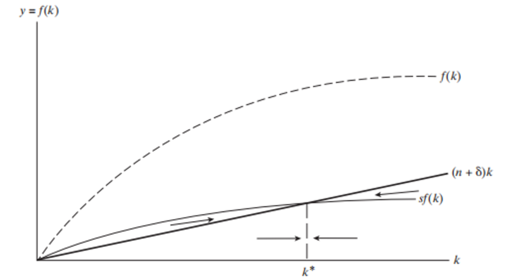
To the left of k*, k<k*, in this case sf(k)>(δ+n)k and as a result, ∆k>0 thus, k is growing towards the equilibrium point k*. To the right of k*, k>k*, in this case sf(k)<(δ+n)k and ∆k<0 and capital per worker is shrinking toward the equilibrium k*.
The equation sf(k*)=(δ+n)k* has an interpretation that the savings per worker, sf(k*) is just equal to δk*, the amount of capital (per worker) needed to replace depreciating capital, plus nk*, the amount of capital (per worker) that needs to be added due to population (labour force) growth.
Effect of Saving in Solow Model
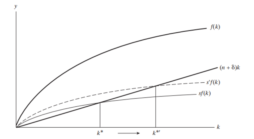
What happens in the Solow neoclassical growth model if we increase the rate of savings, s. An increase in s, leads to temporary increase in the rate of output growth as we increase k by raising the rate of savings. We return to the original steady-state growth rate later, though at a higher level of output per worker in each later year.
The key implication is that unlike in the Harrod-Domar (AK) analysis, in the Solow model an increase in s will not increase growth in the long run; it will only increase the equilibrium k*.
Some Concepts
Capital stock refers to the total amount of physical goods that have been produced at a particular time and are used in the production of other goods and services such as factories, buildings, equipment, plants, etc.
Capital accumulation means increase in country’s stock of real capital (net investment in fixed assets).
Steady-State: Steady state is an equilibrium state where the economy grows at a constant rate, and the capital and output per worker remains constant over time. It can be written as: sf(k*) =(δ+n)k*.
Capital deepening means an increase in the capital–labor ratio (i.e., more capital per worker). It occurs when the growth of capital stock is faster than the growth of labor force.
Capital widening means an increase in the capital stock at the same rate as the labor force, so that the capital–labor ratio remains constant. New capital is added only to equip the growing labor force, not to improve productivity.
Total Factor Productivity (TFP) is the portion of output that cannot be explained by labor and capital. It measures how efficiently and effectively an economy uses its inputs. It is sometimes called Solow residual.
Growth accounting measures the percentage share of an economy`s growth rate explained by the growth rate of labor force, growth rate of capital and residual factors.
Suggestions for further readings:
- Solow’s Model of Growth (With Diagram) – Economics Discussion
