A Numerical Example of Multiple Linear Regression by Hand

Table of Contents

What is Multiple Linear Regression?

The linear regression model shows the linear dependence of one variable on one or more independent variables. A simple linear regression model consists of the linear dependence of one variable on only one independent variable. It is also called a bivariate or two-variable regression model. Such as the dependence of consumption on disposable income.

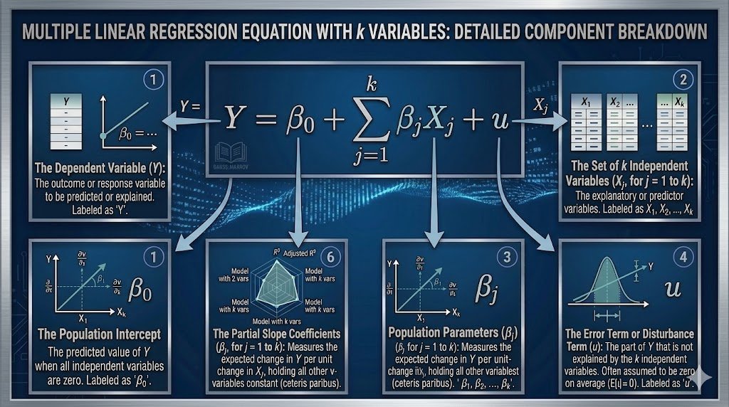
A multiple linear regression model consists of the linear dependence of one variable on two or more independent variables. In other words, in multiple linear regression,, a dependent variable is exprrssed asa linear function of more than one independent variable. It is also called a multivariate regression model. For example, crop yield depends on rainfall, temperature, sunshine, fertilizer, etc. A k-variable multiple linear regression model can be written as:

$Y_i = \beta_0 + \beta_1 X_{1i} + \beta_2 X_{2i} + \cdots + \beta_k X_{ki} + u_i$

$Y_i$ : Dependent variable
$\beta_0$ : Intercept term
$\beta_1, \beta_2, \dots, \beta_k$ : Coefficients of independent variables
$X_{1i}, X_{2i}, \dots, X_{ki}$ : Independent variables
$u_i$ : Error term

To understand multiple linear regression and its interpretation, we consider an example of a 3-variable linear regression model, in which the dependent variable is a linear function of only two explanatory variables. It is written as:

$Y_i = \beta_0 + \beta_1 X_{1i} + \beta_2 X_{2i} + u_i$

A Numerical Example of Multiple Linear Regression

The following table provides data about monthly sales revenue in USD 1000 (Yi), price index for all products sold in a given month (X_1i), and expenditure on advertising in USD 1000 (X_2i).

Obs.	sales	price	advert
1	73.2	5.69	1.3
2	71.8	6.49	2.9
3	62.4	5.63	0.8
4	67.4	6.22	0.7
5	89.3	5.02	1.5
6	70.3	6.41	1.3
7	73.2	5.85	1.8
8	86.1	5.41	2.4
9	81	6.24	0.7
10	76.4	6.2	3
11	76.6	5.48	2.8
12	82.2	6.14	2.7

Answer the following questions.

Estimate and interpret the following model: $Sales_i = \beta_0 + \beta_1 Price_i + \beta_2 Advert_i + \mu_i$
Compute and interpret the multiple coefficient of determination and the multiple standard error of estimate.
Test the significance of regression coefficients and tell whether the signs are according to the underlying theory?
Predict the sales revenue at means.

Solution

1. Estimate and interpret the following model:

. $Sales_i = \beta_0 + \beta_1 Price_i + \beta_2 Advert_i + \mu_i$

The OLS estimates can be obtained by the following formulas.

$\hat{\beta}_1 = \frac{(\sum x_1 y)(\sum x_2^2) - (\sum x_2 y)(\sum x_1 x_2)}{(\sum x_1^2)(\sum x_2^2) - (\sum x_1 x_2)^2}$

$\hat{\beta}_2 = \frac{(\sum x_2 y)(\sum x_1^2) - (\sum x_1 y)(\sum x_1 x_2)}{(\sum x_1^2)(\sum x_2^2) - (\sum x_1 x_2)^2}$

$\hat{\beta}_0 = \bar{Y} - \hat{\beta}_1 \bar{X}_1 - \hat{\beta}_2 \bar{X}_2$

The following identities can be used to find the values in the above formulas.

$\sum x_1 y = \sum X_1 Y - \frac{\sum X_1 \sum Y}{n}$

$\sum x_2 y = \sum X_2 Y - \frac{\sum X_2 \sum Y}{n}$

$\sum x_1 x_2 = \sum X_1 X_2 - \frac{\sum X_1 \sum X_2}{n}$

$\sum x_1^2 = \sum X_1^2 - \frac{(\sum X_1)^2}{n}$

$\sum x_2^2 = \sum X_2^2 - \frac{(\sum X_2)^2}{n}$

$\sum y^2 = \sum Y^2 - \frac{(\sum Y)^2}{n}$

Obs.	Y	X₁	X₂	X₁Y	X₂Y	X₁X₂	X₁²	X₂²	Y²
1	73.2	5.69	1.3	416.508	95.16	7.397	32.3761	1.69	5358.24
2	71.8	6.49	2.9	465.982	208.22	18.821	42.1201	8.41	5155.24
3	62.4	5.63	0.8	351.312	49.92	4.504	31.6969	0.64	3893.76
4	67.4	6.22	0.7	419.228	47.18	4.354	38.6884	0.49	4542.76
5	89.3	5.02	1.5	448.286	133.95	7.53	25.2004	2.25	7974.49
6	70.3	6.41	1.3	450.623	91.39	8.333	41.0881	1.69	4942.09
7	73.2	5.85	1.8	428.22	131.76	10.53	34.2225	3.24	5358.24
8	86.1	5.41	2.4	465.801	206.64	12.984	29.2681	5.76	7413.21
9	81	6.24	0.7	505.44	56.7	4.368	38.9376	0.49	6561
10	76.4	6.2	3	473.68	229.2	18.6	38.44	9	5836.96
11	76.6	5.48	2.8	419.768	214.48	15.344	30.0304	7.84	5867.56
12	82.2	6.14	2.7	504.708	221.94	16.578	37.6996	7.29	6756.84
∑	909.9	70.78	21.9	5349.56	1686.54	129.343	419.768	48.79	69660.4
Mean	75.825	5.89833	1.825	445.796	140.545	10.7786	34.9807	4.06583	5805.03

$\sum x_1 y = \sum X_1 Y - \frac{\sum X_1 \sum Y}{n} = 5349.556 - \frac{(70.78)(909.9)}{12} = -17.3375$

$\sum x_2 y = \sum X_2 Y - \frac{\sum X_2 \sum Y}{n} = 1686.54 - \frac{(21.9)(909.9)}{12} = 25.98$

$\sum x_1 x_2 = \sum X_1 X_2 - \frac{\sum X_1 \sum X_2}{n} = 129.343 - \frac{(70.78)(21.9)}{12} = 0.1695$

$\sum x_1^2 = \sum X_1^2 - \frac{(\sum X_1)^2}{n} = 419.7682 - \frac{5009.8084}{12} = 2.2841$

$\sum x_2^2 = \sum X_2^2 - \frac{(\sum X_2)^2}{n} = 48.79 - \frac{479.61}{12} = 8.8225$

$\sum y^2 = \sum Y^2 - \frac{(\sum Y)^2}{n} = 69660.39 - \frac{827918.01}{12} = 667.2225$

Plugging these values in OLS formula, we get

$\hat{\beta}_1 = \frac{(-17.3375)(8.8225) - (25.98)(0.1695)}{(2.2841)(8.8225) - (0.1695)^2} = \frac{-152.8939 - 4.40361}{20.15 - 0.02873} = -7.82$

$\hat{\beta}_2 = \frac{(25.98)(2.2841) - (-17.3375)(0.1695)}{(2.2841)(8.8225) - (0.1695)^2} = \frac{59.3409 + 2.9387}{20.15 - 0.02873} = 3.094$

$\hat{\beta}_0 = 75.825 - (-7.82)\bar{X}_1 - (3.094)\bar{X}_2$

$\hat{\beta}_0 = 75.825 + 7.82(5.9) - 3.094(1.825)$

$\hat{\beta}_0 = 116.31$

Estimated Regression Equation:

$\hat{Y}_i = 116.31 - 7.82X_1 + 3.094X_2$

2. Compute and interpret the multiple coefficient of determination and the multiple standard error of estimate

Multiple Coefficient of Determination

Formula 1:

$R^2 = \frac{ESS}{TSS} = \frac{\sum (\hat{Y}_i - \bar{Y})^2}{\sum (Y_i - \bar{Y})^2} = \frac{215.937}{667.223} = 0.323$

Formula 2:

$R^2 = \frac{ESS}{TSS} = \frac{\hat{\beta}_1 \sum x_1 y + \hat{\beta}_2 \sum x_2 y}{\sum y_i^2} = \frac{(-7.82)(-17.3375) + (3.094)(25.98)}{667.223} = 0.323$

Multiple Standard Error of Estimate

$SER = \sqrt{\frac{\sum (Y_i - \hat{Y}_i)^2}{n - 3}} = \sqrt{\frac{SSR}{n - 3}} = \sqrt{\frac{451.286}{12 - 3}} = \sqrt{50.1428} = 7.0811$

3. Test the significance of regression coefficients and tell whether the signs are according to the underlying theory.

Standard error and t-value of $\hat{\beta}_1$

$\mathrm{Var}(\hat{\beta}_1) = \frac{\sum x_2^2}{(\sum x_1^2)(\sum x_2^2) - (\sum x_1 x_2)^2} \, \sigma^2$

$\mathrm{Var}(\hat{\beta}_1) = \frac{8.8225}{(2.2841)(8.8225) - 0.02873} \times 50.1428 = 21.98$

$se(\hat{\beta}_1) = \sqrt{\mathrm{Var}(\hat{\beta}_1)} = \sqrt{21.98} = 4.688$

$t_{\hat{\beta}_1} = \frac{\hat{\beta}_1}{se(\hat{\beta}_1)} = \frac{-7.82}{4.688} = -1.668$

Standard error and t-value of $\hat{\beta}_2$

$\mathrm{Var}(\hat{\beta}_2) = \frac{\sum x_1^2}{(\sum x_1^2)(\sum x_2^2) - (\sum x_1 x_2)^2} \, \sigma^2$

$\mathrm{Var}(\hat{\beta}_2) = \frac{2.2841}{(2.2841)(8.8225) - 0.02873} \times 50.1428 = 5.7$

$se(\hat{\beta}_2) = \sqrt{\mathrm{Var}(\hat{\beta}_2)} = \sqrt{5.7} = 2.385$

$t_{\hat{\beta}_2} = \frac{\hat{\beta}_2}{se(\hat{\beta}_2)} = \frac{3.094}{2.385} = 1.297$

4. Predict the sales revenue at mean price and mean advertisement expenditures.

The estimated regression equation is.

$\hat{Y}_i = 116.31 - 7.82X_1 + 3.094X_2$

Substituting the mean values of $X_1$ and $X_2$ , that is plugging $\bar{X}_1 = 5.9$ and $\bar{X}_2 = 1.83$ .

$\hat{Y}_i = 116.31 - 7.82(\bar{X}_1) + 3.094(\bar{X}_2)$

$\hat{Y}_i = 116.31 - 7.82(5.9) + 3.094(1.83)$

$\hat{Y}_i = 116.31 - 46.14 + 5.66$

$\hat{Y}_i = 75.83$

Regression Output Results Summary

$\hat{Y}_i = 116.31 - 7.82X_1 + 3.094X_2$

$se = (27.9,\; 4.688,\; 2.385)$

$t = (4.17,\; -1.668,\; 1.297)$

$R^2 = 0.323,\quad SER = 7.08$

Interpretation of Regression Results

Interpretation of Coefficients and their significance

The regression results show that if the price index of sold goods increases by 1 unit, then sales revenue will decrease by USD 7.8 thousand, holding the advertising expenditure constant. If the advertising expenditure increases by USD 1000, then sales revenue will increase by USD 3000, holding the price index constant. The intercept value shows that the sales revenue is USD 116.3 thousand if the price index of sold goods and advertising expenditure are zero. It makes no sense that if the price index is zero, then the sales revenue is USD 116.3 thousand, because the sales formula is P*Q; if P = 0, then sales must be zero.

The absolute t-value of $\hat{\beta}_1$ is 1.668, which is less than its critical value; therefore, we fail to reject the null hypothesis and conclude that the sales price index has a statistically insignificant effect on sales revenue.

The t-value of $\hat{\beta}_2$ is less than its critical value, so we fail to reject the null hypothesis and conclude that advertising expenditure has no statistically significant impact on sales revenue.

According to the underlying theory, the signs of slope coefficients indicate that an increase in sales price will decrease the demand for the good, leading to a decrease in sales revenue. Similarly, more expenditure on advertising leads to more sales revenue, but the impact of both variables on sales revenue is statistically insignificant.

Interpretation of Multiple R²

The R² value of 0.323 shows that about 32.3% of the variation in sales revenue is explained by the sales price index and advertising expenditure together. While 67.7% of the variation in sales revenue remains unexplained, it is important to consider other factors.

Suggestions for further readings:

Share this article

Muhammad Minhaj Akhtar

Muhammad Minhaj Akhtar is a Lecturer in Economics at Government Graduate College Jauharabad, Pakistan. He holds an M.Phil. in Economics from Quaid-i-Azam University, Islamabad, and an MSc in Economics from the University of Sargodha, where he earned a Silver Medal. His academic passion lies in Econometrics, with a strong focus on applying empirical methods to real-world economic issues. Through MinhajMetrixHub, he shares learning resources, research guidance, and practical econometric insights for students and researchers.

Read Posts

One Response

Pingback: Assumptions of Classical Linear Regression Model (CLRM) - MinhajMetricsHub

A Numerical Example of Multiple Linear Regression by Hand

What is Multiple Linear Regression?

A Numerical Example of Multiple Linear Regression

Share this article

Muhammad Minhaj Akhtar

One Response

Leave a Reply Cancel reply

CATEGORIES

TAGS

Recent Posts

Multicollinearity

Sen Capability Approach

Variance and Standard Error of OLS Estimators and Gauss-Markov Theorem

Assumptions of Classical Linear Regression Model (CLRM)

Regression Through Origin