Econometrics-I Short Questions

Econometrics: Literally, the word econometrics means economic measurement or the measurement of economic relationships. According to Goldberger: Econometrics may be defined as the social science in which the tools of economic theory, mathematics and statistical inference are applied to the analysis of economic phenomena.

Uses/functions/objectives of econometrics:

Testing economic theories and models
Estimating numerical values of economic coefficients
Forecasting future events
Evaluating programs and policies
Identifying cause and effect relationships

Mathematical economics vs econometrics: Mathematical economics concerns expressing economic theory in mathematical form (equations) without measurability or empirical verification of the theory. It expresses the economic relationship in exact or deterministic form. Whereas econometrics empirically tests economic theory or hypothesis and provides estimated values to economic relationships.

Economic statistics vs econometrics: Economic statistics is mainly concerned with collecting, processing, and presenting economic data in the form of charts and tables. Whereas econometrics uses this data to empirically test economic theory or hypothesis. Moreover, econometrics is concerned with causal inference while statistics is mostly concerned with statistical inference.

Cross-sectional data consists of observations collected from various entities such as individuals, households, firms, cities, states and countries at a single point in time. For example, GDP of Asian countries for the year 2023, number of deaths due to coronavirus pandemic in the year 2020. It is often denoted by subscript i.

Time series data consists of observations collected over multiple time periods for a single entity. For example, data about Real GDP, Inflation, Unemployment and Life expectancy of Pakistan from 1991 to 2019. It is often denoted by subscript t.

Pooled (or combined data) have features of both cross section and time series data in which each cross-section unit may not be the same for each time period. For example, data of different students over different semesters and each student may not be the same in each semester.

Panel (or longitudinal) data is a combination of cross-section and time-series data in which data on the same cross-sectional units are collected over multiple time periods. For example, data about GDP, inflation, unemployment rate, money supply, and investment for all developing countries from 1970 to 2023. It is often denoted by subscript it.

Balanced vs unbalanced panel data: In balanced panel number of time observations are same for all cross-section units. There are no missing observations. In unbalanced panel number of time observations are not same for all cross-sectional units. There are missing observations for each cross section.

Primary data is the data collected for the first time by a researcher for his/her specific research purpose. It is collected through surveys, interviews, experiments, observations, and questionnaire. For example, a student collects data from college students to study the relationship between laptop distribution and exam scores.

Secondary data is data that has already been collected by an institution or researcher for different purposes. it can be obtained from sources such as books, reports, articles, online databases and surveys. For example, a student collects data from WDI to study relationship between inflation and unemployment.

Experimental data is collected through controlled experiments where researchers can manipulate one or more independent variables to observe cause-and-effect relationships. For example, testing the effectiveness of a new vaccine.

Non-Experimental data or observational data is collected by observing and recording events, behaviors, or phenomena as they naturally occur without manipulation. This method is used where experiments are not possible, not ethical or expensive. For example, studying the relationship between consumption and income.

Quantitative data is data that can be measured numerically. Such as GDP, GNP, Exports, Prices, Investment etc. Quantitative variables can be classified into two broad categories namely: (i) discrete variables and (ii) continuous variables

Qualitative data or categorical data is the data which cannot be measured numerically but can be classified into several groups or categories. . Such as gender, education level, social status, religion, race etc Categorical data can be nominal or ordinal.

Nominal scale is the lowest level of measurement scale where data is classified into mutually exclusive qualitative categories without ordering or ranking. Examples are gender, colors, house numbers, blood group etc. It is often represented by bar charts or pie charts.

Ordinal scale has the characteristics of nominal scale and in addition has the property of ordering or ranking of categories but the difference between them is not meaningful. For example, the performance of students in class test like excellent, good, fair, poor, very poor or classification of countries based on GNI per capita.

Interval scale has all the characteristics of ordinal level data and the difference between values is also meaningful but the ratios not. It does not have true zero point. For example, temperature recorded for a city over different months.

Ratio scale is the highest level of measurement scale which has all characteristics of interval scale and the ratio between values is also meaningful. It has also a true zero point. For example, income, prices, weight, height, money, output etc.

Regression is a statistical technique which is used to predict the values of one variable based on the values of other variable(s). The variable whose values we want to predict is known as dependent variable (Y) and the variable that explains the variations in the dependent variable is known as independent variable (X).

An economic model is a set of assumptions that describes the behavior of an economy. It consists of mathematical equations that describe various relationships in exact form. Some economic models are circular flow model, business cycle model, demand-supply model etc.

An econometric model is a set of behavioral equations which has two components; one is observed or systematic component and the other is unobserved or unsystematic component. It is used to estimate relationship between dependent and independent variable(s). Linear regression equation is an econometric model.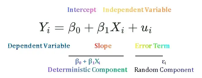

An error term is a term that is included in regression equation to capture the influence of all those variables that affect Y but are not explicitly included in the model. It is denuded by epsilon ε. It is included due to the following reasons: omitted variables, measurement errors, incorrect functional form, or random variations.

The linear regression model shows the linear dependence of one variable on one or more independent variables. The variable whose values we want to predict is known as dependent variable and the variable that explains the variations in the dependent variable is known as independent variable. Example, linear demand function, linear consumption function.

A simple linear regression model consists of linear dependence of one variable on only one independent variable. It is also called bivariate or two variable regression model. Such as dependence of consumption on disposable income.

A multiple linear regression model consists of linear dependence of one variable on two or more independent variables. It is also called multivariate regression model. For example, crop yield depends on rainfall, temperature, sunshine, fertilizer etc.

Deterministic relationships between variables imply exact relationships. It does not include any randomness. If we plot graphs of these relationships, then all data points will lie exactly on the line. Mathematical/economic models are example of deterministic relationships. Y_i = β₀ + β₁ X_i

Stochastic relationships between variables imply inexact or random relationships. If we plot graphs of these models some data points lie above the line, on the line, or below the line. Econometric models are examples of stochastic relationships. Y_i = β₀ + β₁ X_i + u_i

Correlation is a statistical technique which measures the direction and strength of linear relationship between variables. It tells us whether two variables move together in the same direction, move in opposite direction or they are not related. It is measured by correlation coefficient which ranges from -1 to +1.

Conditional vs unconditional mean: Conditional mean is the expected or average value of Y given each fixed values of X written as E (Y | X). Example: Average weekly consumption of a family having a particular income level. Unconditional mean is the expected or average value of Y, but this is not based on the X values written as E (Y). Average weekly family consumption.

Population regression function (PRF) or conditional expected function shows the functional relationship between conditional mean value of dependent variable Yi given the values of independent variable, Xi. When we introduce error term in PRF we get stochastic PRF written as: $Y_i = \beta_0 + \beta_1 X_i + u_i$

Population regression line (PRL) or population regression curve is the locus of conditional means values of dependent variable Y, for each given values of independent variable. More simply, it is the curve connecting the means of the sub populations of Y corresponding to the given values of the regressor X.

Sample regression function (SRF) is the estimated regression equation obtained from a sample of data. It is used to predict the value of the dependent variable given specific values of the independent variables. The linear SRF can be written as: $\hat{Y}_i = \hat{\beta}_0 + \hat{\beta}_1 X_i$

Sample regression line (SRL) is the graphical representation of the sample regression function. It is a line that best fits the scatter plot of the observed data points. The line minimizes the sum of the squared differences between the actual values and the predicted values. It is written as: $\hat{Y}_i = \hat{\beta}_0 + \hat{\beta}_1 X_i$

Estimator and Estimate: An estimator is a rule or formula or method that tells us how to estimate the population parameter from the sample information. A particular numerical value obtained by the estimator is called estimate. Estimator is random whereas estimate is nonrandom.

Error vs Residual: Error is the difference between the actual value of Y in the population and the conditional mean of Y denoted as E (Y |X_i) in the entire population. $u_i = Y_i - E(Y \mid X_i)$ . Residual is the difference between the actual observed value of the dependent variable (Y) and the estimated value of Y, $\hat{Y}_i$ obtained from the sample regression function (SRF), $\hat{u}_i = Y_i - \hat{Y}_i$ .

Least square principle is the mathematical procedure that uses the data to fit a line by minimizing sum of the squared difference between the actual Y values and the predicted values of Y. In other words, least square method chooses the $\hat{\beta}_0$ and $\hat{\beta}_1$ in such a manner that in a given set of data $\sum e_i^2$ is as small as possible.

Numerical properties of OLS estimators:

OLS estimators are expressed as function of X and Y values.
They are point estimators
The mean value of the estimated $\hat{Y}_i$ is equal to the mean value of the actual Y
The mean value of the residuals $Y = \hat{Y}_i$ is zero.
The residuals $Y = \hat{Y}_i$ are uncorrelated with the predicted Y.
The residuals $Y = \hat{Y}_i$ are uncorrelated with X.

Measures of goodness of fit tells us how well the explanatory variable, X, explains the dependent variable, Y. In other words, they measure how well the OLS regression line fits the data. Are the observations tightly clustered around the regression line, or are they spread out? Two most commonly used measures are: Standard Error of Estimate of Regression (SEE or SER) and Coefficient of Determination, R².

Standard error of estimate or regression (SEE or SER) is a measure of goodness of fit. It measures how spread Y values are around the regression line. It is square root of the variance of residuals. The closer the sample values to regression line smaller will be the standard error of regression. $SER = \sqrt{\frac{\sum_{i=1}^{n} (Y_i - \hat{Y}_i)^2}{n - 2}}$

Coefficient of determination is a measure of goodness of fit of regression line. It measures the percentage of the total variation of the dependent variable Y that can be explained by the independent variable, X. It ranges between 0 to 1. $R^2 = \frac{Explained Sum of Squares (ESS)}{Total Sum of Squares (TSS)}$

Properties of coefficient of determination

$r^2$ can never be negative because sum of deviations is always positive.
It ranges between 0 to 1.
If all sample values lie exactly on the sample regression line than $r^2$ would be equal to 1.
If $r^2$ is equal to zero than none of the variation in Y is explained by X.

Share this article

Muhammad Minhaj Akhtar

Muhammad Minhaj Akhtar is a Lecturer in Economics at Government Graduate College Jauharabad, Pakistan. He holds an M.Phil. in Economics from Quaid-i-Azam University, Islamabad, and an MSc in Economics from the University of Sargodha, where he earned a Silver Medal. His academic passion lies in Econometrics, with a strong focus on applying empirical methods to real-world economic issues. Through MinhajMetrixHub, he shares learning resources, research guidance, and practical econometric insights for students and researchers.

Read Posts

Econometrics-I Short Questions

Share this article

Muhammad Minhaj Akhtar

Leave a Reply Cancel reply

CATEGORIES

TAGS

Recent Posts

Education and Economic Development

A Numerical Example of Multiple Linear Regression by Hand

Short Questions Project Appraisal

PMAC-S5-2527-ST1

Capital Budgeting