Permanent Income Hypothesis Explained: Friedman’s Theory of Consumption

Introduction

Imagine two friends. One gets a surprise USD 5,000 bonus at work. The other gets a USD 5,000 permanent raise added to their yearly salary. Both received the same amount of extra money — so why does the first friend spend a little and save the rest, while the second friend starts eating out more, upgrades their phone, and even books a bigger vacation every year? Milton Friedman had a simple explanation: people don’t just react to how much money they have right now — they react to how much money they expect to keep having in the future.

An American economist, Milton Friedman, presented his permanent income theory of consumption in his book A Theory of the Consumption Function in 1957. According to Friedman, consumption is determined by the permanent or long-term expected future income rather than current income.

Friedman argued that households are forward-looking and seek to maintain a stable, smooth standard of living over time, rather than adjusting consumption sharply to every fluctuation in current income.

Human and Non-Human Wealth

Friedman states that permanent income, or expected long-term average income, is earned by human and non-human wealth. Human wealth is earned by providing labor services; therefore, it is also called labor income and investment in human capital like education, health, skills, training, etc. Non-human wealth consists of tangible assets like savings, bonds, shares, real estate, and consumer durables.

Permanent and Transitory Income

Friedman decomposed measured income into two components: permanent income (Yp) and transitory income (Yt). Thus,

$Y_m = Y_p + Y_t$

Permanent Income

Permanent income is the part of income that people expect to persist into the future. Thus, it is the expected long-term average income. The permanent income depends on both human and non-human wealth. Friedman regards permanent income as a weighted sum of current and past incomes. Example: a software engineer expects to earn USD 80,000 annually based on their qualifications and job market conditions.

Transitory Income

Transitory income is temporary income; it is the part of income that people do not expect to persist. Incomes like windfalls, bonuses, lottery winnings, crop failures, temporary unemployment, overtime pay, capital gains, or any other short-lived and unpredictable factor are regarded as transitory income. It can be either positive or negative. Example: the same software engineer receives a USD 10,000 year-end bonus one year, which is not expected to recur regularly.

Put differently, permanent income is average income, and transitory income is the random deviation from that average. Individuals typically adjust their consumption based on permanent income, smoothing out the effects of transitory income fluctuations.

Permanent and Transitory Consumption

Friedman decomposed measured consumption into two components: permanent consumption (Cp), which depends on permanent income, and transitory consumption (Ct), which depends on transitory income. Thus,

$C_m = C_p + C_t$

Permanent Consumption

Permanent consumption is planned consumption consistent with permanent income. It reflects long-term consumption habits and patterns. Example: the software engineer spends USD 50,000 annually on average, which includes regular expenses like rent, groceries, and utilities, based on their expected permanent income.

Transitory Consumption

Transitory consumption refers to temporary, short-term, unplanned, or incidental spending that does not affect the individual’s long-term consumption patterns significantly. Example: upon receiving the USD 10,000 bonus, the engineer decides to take a vacation costing USD 2,000 and save the remaining USD 8,000. This vacation expense is a one-time increase in consumption and does not alter their long-term spending habits.

Assumptions

The hypothesis is based on the following assumptions:

No correlation between transitory income and permanent income.
No correlation between transitory consumption and permanent consumption.
No correlation between permanent income and transitory consumption.
No correlation between transitory consumption and transitory income.
Only permanent income changes affect consumption.

Permanent Income Hypothesis Consumption Function

Friedman’s permanent income hypothesis consumption function is a long-run consumption function which shows the proportional relationship between permanent consumption and permanent income and is a straight line passing through the origin, which implies that APC is constant and is equal to MPC.

$C_p = kY_p$

Average propensity to consume, k (0 < k < 1), depends on the interest rate (i), ratio of non-human to human wealth (w), and individuals’ desire to create wealth (u). Thus,

$k = k(i,w,u)$

Real rate of interest (i): A higher interest rate raises the reward for saving and lowers k.
Ratio of non-human wealth to income (w): A higher wealth-to-income ratio, other things equal, raises k.
Desire to create wealth (u): The more households desire to accumulate wealth, the smaller the k.

We can rewrite our consumption function as:

$C_p = k(i,w,u)Y_p$

To calculate APC, divide both sides by Y.

$APC=\frac{C}{Y}=k\left(\frac{Y_p}{Y}\right)$

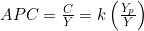
According to the permanent income hypothesis, the average propensity to consume depends on the ratio of permanent income to current income. When current income temporarily rises above permanent income, the average propensity to consume temporarily falls; when current income temporarily falls below permanent income, the average propensity to consume temporarily rises.

Short-Run vs Long-Run APC and MPC

The distinction between permanent and transitory income directly explains why cross-sectional and short-run studies find a declining APC with income, while long-run time-series studies (Kuznets) find a stable APC.

The Short-Run Consumption Function

In a cross-section or a single short period, households with unusually high measured income tend to have received a positive transitory component (Yt > 0), while those with unusually low measured income tend to have experienced a negative transitory shock (Yt < 0). Since transitory income is largely saved, not consumed, the measured APC (C/Y) falls as measured income Y rises — even though the true underlying propensity to consume out of permanent income, k, has not changed. This produces the flatter, positively intercepted short-run consumption function that Keynesian AIH studies observed.

The Long-Run Consumption Function

Over long periods, transitory fluctuations average out to zero for the economy as a whole (E(Yt) = 0), so measured income converges to permanent income (Y ≈ Yp). Consequently, the long-run consumption function becomes C = k·Yp, a proportional (constant-APC) relationship passing through the origin, exactly as Kuznets’s long-run data showed.

Because part of any change in current measured income is transitory, the short-run marginal propensity to consume out of measured income (∂C/∂Y in the short run) is smaller than the long-run MPC, which approaches k as the time horizon lengthens and income changes become permanent.

Short-Run vs Long-Run: A Quick Comparison

Aspect	Short-Run (Cross-Section / Business Cycle)	Long-Run (Secular Growth)
Relationship between Y and Yp	Y often diverges from Yp due to transitory shocks	Y converges to Yp as transitory effects average out
APC (C/Y) behaviour	Declines as income rises	Remains constant (≈ k)
Intercept of C–Y relationship	Positive intercept observed	Approximately zero intercept
MPC out of measured income	Low (since part of ΔY is transitory)	Approximately equal to k (high)

How to Measure Permanent Income

Permanent income cannot be observed directly since it is a subjective, forward-looking expectation. Friedman proposed that permanent income is equal to last year’s income plus a proportion of the change in income that occurred between the last year and the current year. Thus, permanent income can be measured as follows:

$Y_p = Y_{t-1} + a(Y_t - Y_{t-1}), \quad 0<a<1$

$Y_p = Y_{t-1} + aY_t - aY_{t-1}$

$Y_p = aY_t + (1-a)Y_{t-1}$

This last equation shows that permanent income is the weighted average of current and past measured income, with weights declining geometrically as we go further into the past.

Worked Example

Suppose the proportion of change in income between the last year and the current year equals 0.6, and the last year’s income (Yt-1) is Rs. 80,000, and the current year’s income (Yt) is Rs. 85,000. Then, from the equation above, permanent income can be estimated as below:

$Y_p = 0.6(85,000) + (1-0.6)(80,000)$

$= 51,000 + 32,000$

$= 83,000$

Graphical Presentation of Permanent Income Hypothesis

In the short run, the consumption function is linear and non-proportional, i.e., APC > MPC, and in the long run, the consumption function is linear and proportional, i.e., APC = MPC. Consumers would move along the long-run consumption curve if the increase in income is permanent, and move along the short-run consumption curve if the increase in income is temporary.

Figure 1: Permanent Income Hypothesis Consumption Function

Permanent Income Hypothesis

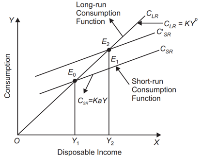
Explanation: Figure 1 shows that C_SR and C_‘SR are short-run consumption functions, whereas C_LR is the long-run consumption function. At OY₁ income level, where C_SR and C_LR curves coincide at point E₀, permanent income and measured income are identical, and so are permanent and measured consumption, as shown by Y₁E₀. If the increase in income is temporary, then the consumer moves from point E₀ to E₁. Thus, consumption increases from Y₁E₀ to Y₂E₁, but if the increase in income is permanent, then the short-run consumption function shifts upward onto the long-run consumption function, and thus, there would be a permanent increase in consumption. Thus, he increases his consumption from Y₁E₀ to Y₂E₂.

Limitations

Ignores correlation between temporary income and consumption.
APC is not the same for all social groups.
No clear distinction between human and non-human wealth.
Difficult to measure permanent income.
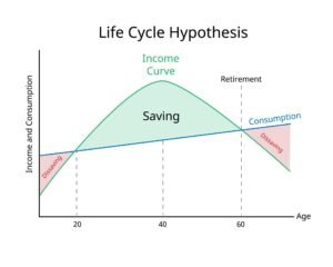
Ignores life cycle factors like retirement, family formation, and demographic factors like age, etc.
It assumes rationality and forward-looking individuals, but not every individual cares about permanent income.
In developing countries, people do not plan their consumption or income due to financial illiteracy.

Comparing PIH with AIH and RIH

Feature	Absolute Income Hypothesis (Keynes)	Relative Income Hypothesis (Duesenberry)	Permanent Income Hypothesis (Friedman)
Main determinant of consumption	Current absolute income	Relative income position & past peak consumption	Long-run permanent (expected) income
APC as income rises	Falls	Falls in short run for individual; economy-wide APC can be stable	Constant (= k) with respect to permanent income
Time horizon	Short run / current period	Habit-based, backward-looking	Forward-looking, long horizon
Reaction to temporary income changes	Consumption changes roughly proportionally	Limited by habit persistence (ratchet effect)	Largely saved; little effect on consumption
Explains Kuznets puzzle?	No (predicts falling long-run APC)	Partially (via demonstration effect / ratchet)	Yes — directly and completely

FAQs

Q1. What is the Permanent Income Hypothesis?
The Permanent Income Hypothesis, proposed by Milton Friedman in 1957, states that a household’s consumption is based on its expected long-term average (permanent) income rather than its current measured income.

Q2. What is the difference between permanent income and transitory income?
Permanent income is the long-term expected average income from human and non-human wealth, while transitory income is a temporary, unpredictable deviation from that average, such as a bonus or windfall gain.

Q3. What is the Permanent Income Hypothesis consumption function?
It is expressed as Cp = kYp, showing a proportional relationship between permanent consumption and permanent income, where k is the average propensity to consume out of permanent income.

Q4. How does the Permanent Income Hypothesis explain the Kuznets puzzle?
Since transitory income fluctuations average out to zero over the long run, measured income converges to permanent income, producing a stable, proportional consumption function — exactly what Kuznets observed in long-run data.

Q5. What are the main limitations of the Permanent Income Hypothesis?
Its key limitations include the difficulty of measuring permanent income, ignoring life-cycle factors, assuming full rationality, and overlooking financial illiteracy in developing countries.

Suggestions for further readings

Permanent Income Hypothesis Explained: Friedman’s Theory of Consumption