

Various Functional Forms of Regression Models
Double-Log Model Explained with Examples
Introduction
Regression analysis is one of the most powerful tools in econometrics, but a model is only as good as its functional form. Choosing the wrong functional form does not just produce a slightly different result — it can completely change how a coefficient should be interpreted, distort the meaning of elasticity, and lead to biased and misleading conclusions about the underlying economic relationship.
Most students are first introduced to the simple Linear Regression Model (Lin-Lin Model), where both the dependent variable (Y) and the independent variable (X) appear in their original, untransformed form. While this model is easy to interpret, it assumes a constant slope and a non-constant elasticity, which is often unrealistic in real economic settings such as demand functions, production functions, or wage equations.
This article explains one of the three most widely used alternative functional forms in econometrics — the Double-Log Model, along with its derivations, interpretation rules, real-world applications, and fully worked numerical examples.
While other functional forms like the Log-Lin Model and the Lin-Log Model will be discussed in the next article. By the end of a couple of articles, students will be able to identify which functional form fits a given economic relationship and interpret the regression coefficients correctly.
Why Functional Forms Matter in Econometrics
The correct functional form determines three critical things:
- How the slope coefficient should be interpreted
- What the elasticity actually means
- Whether the model is correctly specified
A misspecified functional form leads to biased and misleading parameter estimates, even if the estimation technique (such as Ordinary Least Squares) is applied correctly. This is why economic theory, combined with visual inspection of scatter plots, should always guide the choice of functional form before estimation begins.
The Linear Regression Model (Lin-Lin Model) — A Quick Recap
Also known as the Baseline Model, the Lin-Lin model estimates a linear relationship between a dependent variable and one or more independent variables, where both Y and X remain in their original (level) form — no transformation is applied to either variable. It is typically estimated using Ordinary Least Squares (OLS), which minimizes the Sum of Squared Residuals (SSR).
The linear regression model can be written as:

Key properties of the Linear model:
- The slope coefficient (β₁) is constant at all values of X and Y. A one-unit increase in X leads to a β₁-unit change in Y, on average.
- The elasticity is NOT constant — it varies with the values of X and Y, since elasticity equals β₁ multiplied by (X/Y). That is
 .
.
 .
.Example: If Y is the quantity demanded of wheat (in kg) and X is the price per kg of wheat (in USD), and β₁ = −0.8, then every USD 1 increase in price leads to a 0.8 kg decrease in the quantity demanded of wheat, on average.
Because the Lin-Lin model cannot capture constant elasticities or relationships that involve elasticities or semi-elasticities, economists frequently turn to logarithmic transformations of Y and/or X. This gives rise to three important functional forms:
- Double-Log or Log-Linear Models
- Log-Lin or Growth Models
- Lin-Log
The Double-Log Model (Log-Log Model)
Definition and General Form
The Double-Log Model, also called the Log-Log Model or Log-Linear Model, transforms both the dependent variable Y and the independent variable(s) X into their natural logarithms. Because the resulting equation is linear in the logarithms of Y and X, it can be estimated directly using OLS without any special modification.
General Form:

Why It Is Called “Log-Log” or “Log-Linear”
- Log-Log Model: because both Y and X are expressed in log form.
- Log-Linear Model: because the model is linear in the logs of Y and X, even though the original relationship between Y and X may be non-linear.
Derivation of the Slope and Elasticity
Starting Model

Differentiate both sides with respect to X

Multiply both sides by Y

Elasticity Formula

Substitute the slope

Simplify

Final Result

Conclusion
- The slope (dY/dX) equals β₁ multiplied by (Y/X) — this is NOT constant; it changes depending on the values of Y and X.
- The elasticity (ε), defined as (dY/dX) multiplied by (X/Y), simplifies directly to β₁ – and this is constant across all values of X and Y.
This is precisely why the Double-Log model is also called the Constant Elasticity Model.
Interpreting the Slope Coefficient β₁
Formal Derivation of Interpretation
From the slope in a double-log model

Rearrange

Express as the ratio of proportional changes

Multiply numerator and denominator by 100
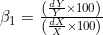
Interpretation in percentage terms
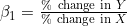
Final interpretation

In the double log model, since the slope coefficient directly measures elasticity, that is, β₁ equals the percentage change in Y divided by the percentage change in X. Therefore, the slope coefficient measures the elasticity of Y w.r.t X (if there is simple regression, i.e., only one independent variable). If there were more than one independent variable, then the slope coefficients would measure partial elasticities of Y w.r.t particular X.
Interpretation Rule: If X increases by 1%, then Y changes by β₁ percent on average, holding other variables constant.
Sign and magnitude interpretation:
- β₁ > 0 — Positive relationship: a 1% increase in X leads to a β₁% increase in Y.
- β₁ < 0 — Inverse relationship: a 1% increase in X leads to a |β₁|% decrease in Y.
- β₁ = 1 — Unit elastic
- β₁ > 1 — Elastic
- β₁ < 1 — Inelastic
Applications of the Double-Log Model
The Double-Log model is preferred whenever economic theory predicts a constant elasticity relationship between Y and X. Common applications include:
- Demand Functions — Income elasticity of demand (% change in quantity demanded for a 1% change in consumer income) and price elasticity of demand (% change in quantity demanded for a 1% change in price).
- Production Functions — Labor elasticity of output (% change in output for a 1% change in labor) and capital elasticity of output (% change in output for a 1% change in capital).
- Returns to Scale in Multi-Input Models — In a Cobb-Douglas production function with two inputs, the sum of the estimated coefficients (
 ) measures returns to scale.
 ) measures returns to scale.
Worked Example 1: Cobb-Douglas Production Function
Mexican Economy (1955–1974)
Consider the following model of the Mexican economy

| Variable | Definition | Economic Role |
|---|---|---|
| Yₜ | Gross Domestic Product (GDP) | Dependent variable |
| X₁ₜ | Labor (thousands of people) | Independent variable — labor input |
| X₂ₜ | Capital (million pesos) | Independent variable — capital input |
| β₁ | Partial elasticity of output w.r.t. Labor | Coefficient on labor |
| β₂ | Partial elasticity of output w.r.t. Capital | Coefficient on capital |
The estimated model is:

Interpretation:
- Labor Elasticity of Output (β̂₁ = 0.3397): If labor increases by 1%, GDP increases by approximately 0.34% on average, holding capital constant.
- Capital Elasticity of Output (β̂₂ = 0.846): If capital increases by 1%, GDP increases by approximately 0.85% on average, holding labor constant. Capital contributes more to output than labor in the Mexican economy.
- R² = 0.995 indicates that the log of labor and the log of capital together account for 99.5% of the variation in the log of real GDP.
- F = 1719.23 shows that the overall model is significant (compare the F-statistic with 4, the rule of thumb at a 5% significance level).
Returns to Scale:
| Condition | Interpretation |
|---|---|
| β̂₁ + β̂₂ = 1 | Constant Returns to Scale (CRS) |
| β̂₁ + β̂₂ > 1 | Increasing Returns to Scale (IRS) |
| β̂₁ + β̂₂ < 1 | Decreasing Returns to Scale (DRS) |
Total elasticity with respect to both inputs is:

Since β̂₁ + β̂₂ = 1.19, which is greater than 1, the Mexican economy exhibits Increasing Returns to Scale (IRS) during this period.
Worked Example 2: Energy Demand Function
7 OECD Countries (1960–1982)
Consider the following model of 7 OECD countries
Where
- Y = Index of aggregate final energy demand
- X₁ = Index of real GDP
- X₂ = Index of real energy price
And the estimated model is:

Interpretation:
- Income Elasticity (β̂₁ = 0.9972): If real GDP increases by 1%, energy demand increases by approximately 0.9972% (almost exactly 1%), holding energy price constant. This is approximately unit elastic.
- Price Elasticity (β̂₂ = −0.3315): If real energy price increases by 1%, energy demand falls by approximately 0.33%, holding real GDP constant. Since the absolute value is less than 1, energy demand is inelastic with respect to price.
- R² = 0.994 indicates that the log of real GDP and the log of real energy price together account for 99.4% of the variation in the log of energy demand.
- F = 1688.23 shows that the overall model is significant (compare the F-statistic with 4, the rule of thumb at a 5% significance level).
Taking the Natural Log of a Series in Excel, Stata, and Eviews
Since all three functional forms above rely on natural log transformations, it is essential for students to know how to generate a log series in commonly used statistical software.
Taking Natural Log in MS Excel
Follow these steps to generate a natural log series in Excel:
- Open your dataset in Excel and identify the column containing the variable you want to transform (for example, column B contains “GDP”).
- Click on an empty cell in the row next to your first data point (for example, cell C2).
- Type the formula: =LN(B2)
- Press Enter. This returns the natural logarithm of the value in cell B2.
- Click on cell C2 again, then drag the fill handle (the small square at the bottom-right corner of the cell) down through the rest of your data rows to apply the formula to the entire column.
- Label column C as “lnGDP” (or the appropriate variable name) for clarity.
Note: The Excel function LN() returns the natural logarithm (base e), which is exactly what is required for Double-Log, Log-Lin, and Lin-Log regression models. Do not use the LOG10() function, as it returns the base-10 logarithm.
Watch Video to Take Natural Log In Excel
Taking Natural Log in Stata
- In Stata, the natural log of a variable can be generated using the generate command combined with the ln() function: generate lnGDP = ln(GDP)
- If you want to generate log variables for multiple variables at once, you can repeat the command for each variable:
generate lnLabor = ln(Labor)
generate lnCapital = ln(Capital) - To generate the log of a variable while replacing an existing variable, use:
replace lnGDP = ln(GDP)
Taking Natural Log in Eviews
In Eviews, the natural log of a series can be generated in two ways:
Method 1 — Using the Generate (Genr) command:
genr lnGDP = log(GDP)
Method 2 — Using the Object menu (GUI method):
- Open the workfile containing your series.
- Click on Quick from the top menu, then select Generate Series.
- In the dialog box, type: lnGDP = log(GDP)
- Click OK. Eviews will automatically create a new series named “lnGDP” containing the natural log values.
Note: In Eviews, the function log() returns the natural logarithm (base e), not the base-10 logarithm. This matches the LN() function in Excel and the ln() function in Stata.
FAQs
1. What is the main difference between the Double-Log, Log-Lin, and Lin-Log models?
The Double-Log model transforms both Y and X into logs and gives a constant elasticity. The Log-Lin model transforms only Y into log form and measures the percentage change in Y for a one-unit change in X. The Lin-Log model transforms only X into log form and measures the absolute change in Y for a percentage change in X.
2. Why is the Double-Log model called the Constant Elasticity Model?
Because in the Double-Log model, the elasticity of Y with respect to X simplifies exactly to the slope coefficient β₁, which does not vary with the values of X or Y — making the elasticity constant at every point on the regression line.
3. How do you interpret the slope coefficient in a Log-Lin model?
In a Log-Lin model, multiplying the slope coefficient by 100 gives the approximate percentage change in Y for a one-unit increase in X, holding other variables constant. This is why the Log-Lin model is also called the Growth Rate Model.
4. What does Returns to Scale mean in a Cobb-Douglas production function?
Returns to scale is measured by summing the partial output elasticities of labor and capital (β̂₁ + β̂₂) in a Double-Log Cobb-Douglas model. A sum equal to 1 indicates Constant Returns to Scale, greater than 1 indicates Increasing Returns to Scale, and less than 1 indicates Decreasing Returns to Scale.
5. Which functional form is used for Engel curves in economics?
Engel curves, which describe how expenditure on a good changes with income, are typically estimated using the Lin-Log model, since it captures the diminishing absolute effect of a percentage increase in income (or total expenditure) on the level of expenditure for a specific good.
Suggestions for Further Readings:






 MinhajMetricsHub
One response to “Functional Forms of Regression Models: The Double-Log Model in Econometrics”
[…] the previous article, we examined the Double-Log Model, where both the dependent and independent variables are expressed in logarithmic form, […]