

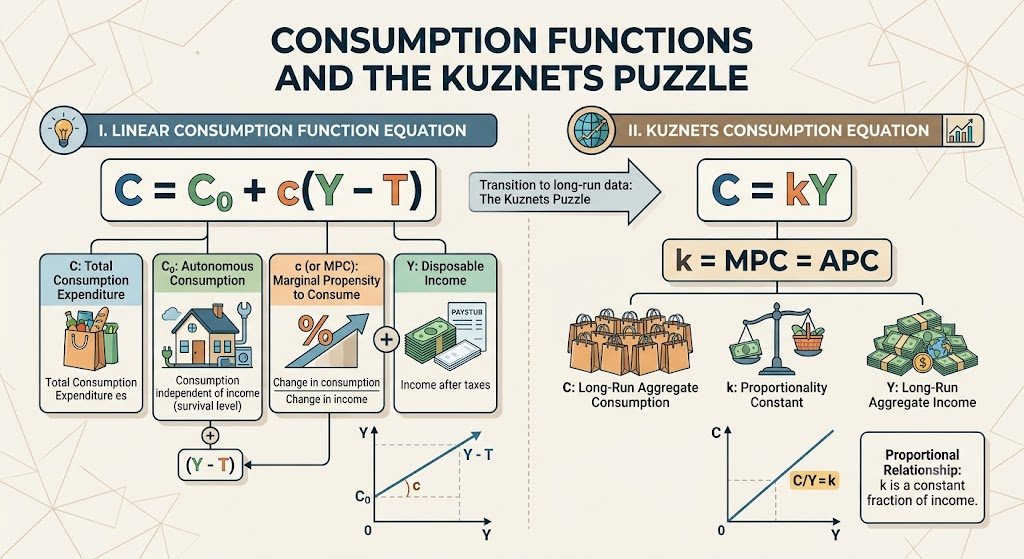
In macroeconomic analysis, consumption is one of the most important components of aggregate demand and plays a fundamental role. Economists have developed a number of ideas that explain how individuals and households make consumption decisions. Households must decide how much to consume now and how much to save for later use.
In this blog post, we discuss the Psychological Law of Consumption of Keynes which is the foundation of all later consumption theories, Keynesian Consumption Function, the Kuznets’ Consumption Function and the famous Kuznets’ Consumption Puzzle and their assumptions, diagrams and important differences.
Keynesian Psychological Law of Consumption
Introduction to Psychological Law of Consumption
Keynes in his book “The General Theory of Employment, Interest and Money”, 1936, postulated that aggregate consumption is a function of aggregate current disposable income. The concept of consumption function plays an important role in Keynes’s theory of income and employment His theory of consumption is also known as the absolute income theory.
Statement of the law
The relation between consumption and income is based on his fundamental psychological law of consumption, which states that “People on average increase their consumption as their income increases, but not by as much as the increase in their incomes.”
Three Related Propositions of Psychological Law of Consumption
Proposition 1
When the aggregate income increases, consumption expenditure also increases, but by a somewhat smaller amount. The cause is that as income increases, our wants have already been satisfied, so there is less need to increase consumption in proportion to the increase in income. Thus, ∆C < ∆Y.
Proposition 2
An increase in income is divided in some proportion between consumption expenditure and saving. It means that income increases will either be consumed or saved. Thus, ∆Y = ∆C + ∆S.
Proposition 3
With the increase in income, both consumption spending and savings increase. Thus, ∆C/∆Y>0 and ∆S/∆Y>0
Explanation with the help of schedule and diagram
Table 1: Proposition of Keynes’s Law
| Income (Y) | Consumption (C) | Saving (S) |
| 0 | 40 | -40 |
| 100 | 120 | -20 |
| 200 | 200 | 0 |
| 300 | 280 | 20 |
| 400 | 360 | 40 |
| 500 | 440 | 60 |
| 600 | 520 | 80 |
Explanation
Table 1 explains Keynes propositions. Firstly, ∆C < ∆Y. At each 100 units increase in income leads to increase consumption by 80 units. Secondly, ∆Y=∆C+ ∆S. At each increase in income of 100 units is divided 80 units and 20 units increase in consumption and saving respectively. Finally, ∆C/∆Y>0, ∆S/∆Y>0, when income increases from 0 to 600 units, consumption and savings also increase from 40 to 520 and -40 to 80 units respectively.
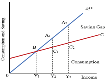
Figure 1: Keynes Three Propositions
Explanation:
Figure 1 explains three Keynes propositions. Firstly, ∆C < ∆Y; this can be shown when income increases from OY1 to OY2, consumption also increases from BY1 to C1Y2, but the increase in consumption is less than the increase in income, i.e., C1Y2 < A1Y2. Secondly, ∆Y=∆C+ ∆S When income increases to OY2 and OY3, it is divided in some proportion between consumption C1Y2 and C2Y3 and saving A1C1 and A1C2, respectively. Finally, ∆C/∆Y>0 and ∆S/∆Y>0. An increase in income from OY2 to OY3 led to increased consumption (C2Y3>C1Y2) and increased saving (A2C2>A1C1) compared to before.
Absolute Income Hypothesis
Introduction
Keynes argued that absolute income is an important factor that determines the consumption of society. Absolute income means actual current income. Keynes’s approach to the consumption function is called the ‘absolute income hypothesis’, which is based on Keynes’s psychological law of consumption.
Keynes Psychological Law of Consumption
This law explains the consumption behaviour of people, which states that “people on average increase their consumption as their income increases, but not by as much as the increase in their incomes.” That is,
0<MPC<1
Important Features of Keynes’s Consumption Function
- First, absolute level of current income is the primary determinant of consumption. Increase in national income causes an increase in consumption and vice versa. However Classical economists considered rate of interest a primary determinant of consumption.
- Second, marginal propensity to consume (MPC) is between 0 and 1. It is due to the Keynes psychological law of consumption. As income increases, consumption increases but not as much as the increase in income.
- Third, as income rises APC tends to fall. It is because at higher income people save large portion of their income. Falling APC implies that the consumption function is non-proportional
- Fourth, Keynes consumption function remains stable in the short run, that is, it does not shift upward or downward. Keynes argued that various institutional factors such as
- Distribution of income and wealth across households
- Financial institutions and credit availability
- Government taxation and welfare systems
- Social norms around spending and saving
And psychological factors:
- Willingness and desire to save (thrift)
- Precautionary saving motives (rainy day funds)
- Myopia: preference for present over future consumption
- Expectations of future income
Those effects on consumption are stable in the short run.
Mathematical Explanation
Based on the above features, Keynes’ consumption function can be written as:



Where C is consumption, Y is disposable income, C0 is autonomous consumption, C0>0, and c is the marginal propensity to consume, it is the slope of the consumption function.
Tabular and Diagrammatical Explanation
Table 2: Keynesian Consumption Function
| Income (USD) | Consumption (USD) | APC=C/Y | MPC=∆C⁄∆Y |
| 1000 | 950 | 0.95 | — |
| 1100 | 1020 | 0.93 | 0.7 |
| 1200 | 1090 | 0.91 | 0.7 |
| 1300 | 1160 | 0.89 | 0.7 |
| 1400 | 1230 | 0.88 | 0.7 |
| 1500 | 1300 | 0.87 | 0.7 |
| 1600 | 1370 | 0.86 | 0.7 |
| 1700 | 1440 | 0.85 | 0.7 |
| 1800 | 1510 | 0.84 | 0.7 |
Explanation: Table 2 shows the three properties of the Keynesian consumption function.
- Consumption rose from 950 to 1510 as income increased from 1000 to 1800.
- MPC is between 0 and 1; in this case, MPC = 0.7.
- APC is declining from 0.95 to 0.89 as income rises.
Figure 2: Keynesian Consumption Function
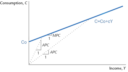
Explanation: The curve C’C’ is a consumption function that rises upwards. The slope of this consumption function is the MPC, which is 0.7. APC is declining; it is shown by the slope of dashed lines drawn from the origin to the consumption function, which becomes flatter as income increases.
Criticism of Keynes Consumption Function
- Kuznets Paradox: Simon Kuznets (1946) found APC remained constant in the long run contradicting Keynes’s prediction that APC falls as income rises.
- Ignores Relative Income: James Duesenberry (1949) argued that consumption depends on relative income, not on absolute income.
- Ignores Permanent Income: Milton Friedman (1957) states that consumption depends on permanent (long-run average) income.
- Ignores Life-Cycle Effects: Franco Modigliani (1954) argued that consumption depends on lifetime earnings.
Kuznets Consumption Function and Kuznets Consumption Puzzle
Introduction
Simon Kuznets (a Nobel Laureate) in 1946 empirically tested the Keynesian consumption function by taking the U.S data on aggregate consumption and income for the period of 1869 to 1933.
Kuznets Findings
Kuznets’s (1946) findings suggested the long-run behaviour of consumers might differ from their short-run consumption patterns. His results showed that APC remained constant during this time period, which was nearly 0.9. Further, he divided the 1869 to 1933 period into three overlapping subperiods and found that APC is the same and equal to about 0.87. Thus, there exists a proportional relationship between consumption and income over this long time period.
Kuznets Consumption Function
This finding suggests a consumption function of the form.
C = kY
This equation implies that MPC = APC = K. Further, the value of the MPC is much higher in Kuznets’s function compared to Keynes’s. Quantitatively, we can write the Kuznets consumption function as:
C = 0.9 Y
Figure 3: Kuznets Consumption Function
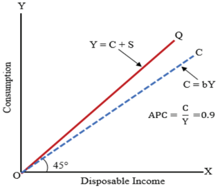
Explanation: Figure 2 shows Kuznets’ proportional consumption function. APC=0.9, which is constant over a long period of time. Line Z is an equality line which shows that Y=C+S. The consumption function is close to a 45-degree line, which suggests that MPC is higher in the Kuznets Consumption function compared to the Keynes consumption function.
The Kuznets Consumption Puzzle or Kuznets Paradox
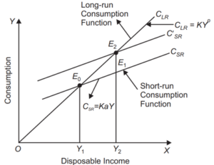
Keynes suggested that APC falls with the rise in income, i.e., MPC < APC in the short run, while Kuznets found that APC is constant, which implies that APC = MPC in the long run. Thus, there are two consumption functions, one for the short run and the second for the long run. Economists called this contradiction between the Keynesian and Kuznets consumption functions a consumption puzzle. It can be illustrated by the following diagram.
Figure 4: The Consumption Puzzle.
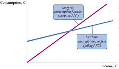
Explanation: Figure 4 shows two consumption functions, one for households’ data and a short time series in which APC is falling with the income, and the slope, which is MPC, is less than APC. Second, for the long time series in which APC is constant and starts from the origin, MPC is equal to APC.
Difference between Keynesian and Kuznets consumption functions
Table 3: Difference between Keynesian and Kuznets consumption functions
| Feature | Keynesian CF (AIH) | Kuznets CF |
| Time Horizon | Short run | Long run |
| Type | Non-proportional | Proportional |
| Equation | C = C₀ + cY | C = kY |
| Autonomous Consumption | C₀ > 0 (positive intercept) | C₀ = 0 (no intercept) |
| Passes Through Origin? | NO — CF starts above origin | YES — CF starts at origin (0,0) |
| MPC | c = 0.70 (constant slope) | k = 0.90 (constant slope) |
| APC | APC = C₀/Y + c → FALLING | APC = k = CONSTANT = 0.9 |
| Relationship (MPC & APC) | MPC < APC (always) | MPC = APC = k |
| Data Source | Household cross-section data | 65 years US aggregate time-series |
| Based on | Psychological law of consumption | Empirical testing of US data (1946) |
| Policy Implication | Rich save more → higher MPS | Saving rate constant across income levels |
Suggestions for Further Readings



 MinhajMetricsHub
6 responses to “Absolute Income Hypothesis”
[…] Absolute Income Hypothesis […]
[…] Absolute Income Hypothesis […]
[…] Absolute Income Hypothesis […]
[…] point of any econometric study is a testable statement derived from economic theory. According to Keynes’s Absolute Income Hypothesis, as disposable income rises, households increase their consumption expenditure, but by a smaller […]
[…] Maynard Keynes, in his Absolute Income Hypothesis, was the first to study this question closely. He said that spending depends on current income and […]
[…] Absolute Income Hypothesis assumes that current consumption depends only on current income. In this view, the future does not […]