

Functional Forms of Regression Models
The Semi-Log Model in Econometrics
In the previous article, we examined the Double-Log Model, where both the dependent and independent variables are expressed in logarithmic form, allowing coefficients to be interpreted as elasticities. However, not all economic relationships exhibit constant elasticity, making other functional forms more appropriate in certain situations.
This article introduces two important semi-logarithmic models: the Log-Lin Model and the Lin-Log Model. The Log-Lin Model is used when a one-unit change in an independent variable causes a percentage change in the dependent variable, while the Lin-Log Model is suitable when a percentage change in an independent variable leads to a constant absolute change in the dependent variable.
We will discuss the mathematical form, coefficient interpretation, elasticity, practical applications, and numerical examples of both models. By the end of this article, students will be able to distinguish between the Log-Lin, Lin-Log, and Double-Log Models and interpret their regression coefficients correctly.
Semi-Log Models: An Overview
In Semi-Log models, only one variable — either Y or X — is transformed into logarithmic form, while the other remains linear. This produces two distinct types of semi-log models, each with a different slope interpretation:
| Model | Y | X | Interpretation of β₁ |
|---|---|---|---|
| Log-Lin | Logarithmic | Linear | 100 × β₁ = % change in Y for a 1-unit change in X |
| Lin-Log | Linear | Logarithmic | β₁ ÷ 100 = absolute change in Y for a 1% change in X |
Key distinction: In the Log-Lin model, the slope measures the relative (percentage) change in Y for an absolute change in X. In the Lin-Log model, the slope measures the absolute change in Y for a relative (percentage) change in X.
The Log-Lin Model (Growth Rate Model)
Definition and Derivation
In the Log-Lin Model, Y is expressed in natural log form while X remains in its original linear form. This model is widely known as the Growth Rate Model, because it is commonly used to estimate the compound growth rate of an economic variable over time.
General Form:

Derivation of Slope, Elasticity, and Semi-Elasticity
Differentiate ln Y w.r.t. X:

Rearrange for the slope:

Slope is not constant:

Elasticity formula:

Substituting the slope:

Elasticity varies with X:

Semi-elasticity interpretation:
We know that , rearrange it for β₁

Percentage interpretation:

Thus, we found that
- The slope (dY/dX) equals β₁ multiplied by Y — this is NOT constant.
- The elasticity (ε) equals β₁ multiplied by X — this also varies with X.
- The semi-elasticity, however, is constant: 100 × β₁ gives the percentage change in Y for a one-unit change in X.
Interpretation Rule: 100 × β₁ equals the percentage change in Y for a ONE-UNIT increase in X, ceteris paribus.
Applications of the Log-Lin Model
- Growth Rate Models — Estimating the annual growth rate of economic variables such as GDP, output, or money supply. Here, β₁ × 100 gives the percentage growth rate per unit of time (e.g., per year).
- Population Growth Equations — Where β₁ × 100 gives the annual population growth rate, and the antilog of the intercept gives the initial population level.
- Returns to Education (Mincerian Earnings Equation) — Where β₁ × 100 estimates the percentage increase in wages for each additional year of schooling.
Important Note: In the Log-Lin model, the elasticity (ε = β₁ · X) varies with X, unlike the Double-Log model, where elasticity is constant. The Log-Lin model instead gives a constant semi-elasticity (β₁), not a constant elasticity.
Worked Example 1: US Population Growth (1975–2007)
Model Specification

Estimated Equation

Interpretation of the coefficient (0.0107):

Interpretation:
- Annual Population Growth Rate: 100 × 0.0107 = 1.07% per year. The US population grew at an annual rate of approximately 1.07% during 1975–2007.
- Initial Population Level: The intercept represents ln(Population) when time = 0, i.e., at the end of 1974, the start of the sample. Taking the antilog, e^5.3593 ≈ 212.57 million, which is the estimated US population at the beginning of the sample period.
Worked Example 2: Mincerian Earnings Function
Returns to Education and Experience
Model Specification:

The natural log of wages is regressed on years of education (X₁) and years of experience (X₂).
Estimated Model


Percentage Interpretation of X1 and X2
Interpretation:
- Returns to Education (β̂₁ = 0.104): An additional year of education increases wages by approximately 10.4% (100 × 0.104 = 10.4%) on average, holding experience constant.
- Returns to Experience (β̂₂ = 0.014): An additional year of experience increases wages by approximately 1.4% (100 × 0.014 = 1.4%) on average, holding education constant.
- R² = 0.277 means education and experience jointly explain 27.7% of the variation in log wages.
The Lin-Log Model
Definition and Derivation
In the Lin-Log Model, Y remains in its original linear form while X is transformed into natural log form. This model is used when the researcher is interested in the absolute change in Y resulting from a relative (percentage) change in X.
General Form:

Differentiate with respect to X
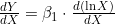
Since d(ln X) = dX/X

Slope

Slope is not constant

Elasticity Formula
Substituting the slope

Elasticity varies with Y

Interpretation Rule

More precise interpretation

Thus, we have found that:
- The slope (dY/dX) equals β₁ multiplied by (1/X) — this is NOT constant.
- The elasticity (ε) equals β₁ divided by Y — this varies with Y.
Interpretation Rule: β₁ ÷ 100 equals the absolute change in Y for a ONE PERCENT increase in X, ceteris paribus.
Worked Example 1: Engel Curve
Food Expenditure (869 US Households, 1995)
Model Specification:

The share of food expenditure (Expfood) is regressed on the natural log of total household expenditure (Expend).
Estimated equation results:

Interpretation:
- Rule: β̂₁ ÷ 100 = absolute change in Expfood for a 1% increase in Expend.
- If total expenditure increases by 1%, the food expenditure share falls by USD 0.00077 (−0.077 ÷ 100) on average. Or if total expenditure increases by 100%, the food expenditure share falls by USD 0.077 on average.
- This result confirms Engel’s Law: as income rises, the budget share spent on food — a necessity good — declines, which is consistent with a negative β̂₁.
Worked Example 2: Life Expectancy and Health Expenditure
Pakistan (2000–2023)
Model Specification:

Life expectancy (LE) is regressed on the natural log of current health expenditure.
Estimated equation results:


Interpretation:
- Rule: β̂₁ ÷ 100 = absolute change in LE for a 1% increase in health expenditure.
- If health expenditure increases by 1%, life expectancy increases by approximately 0.041 years (4.077 ÷ 100 = 0.04077) on average — roughly 15 days, or half a month.
- R² = 0.803 indicates that the log of health expenditure explains 80.3% of the variation in life expectancy in Pakistan during this period.
- F = 90.14, which is very high, indicates that the overall model is statistically significant.
Summary — Comparing All Four Functional Forms
| Model | Slope (dY/dX) | Elasticity (ε) | What β₁ Measures |
|---|---|---|---|
| Lin-Lin (Linear) | β₁ — constant | β₁·(X/Y) — varies | Absolute ΔY per unit ΔX |
| Log-Log (Double-Log) | β₁·(Y/X) — varies | β₁ — constant | % ΔY per 1% ΔX (elasticity) |
| Log-Lin | β₁·Y — varies | β₁·X — varies | % ΔY per unit ΔX (×100) |
| Lin-Log | β₁/X — varies | β₁/Y — varies | Absolute ΔY per 1% ΔX (÷100) |
Key takeaway: Only the Lin-Lin model has a constant slope, and only the Double-Log model has a constant elasticity. All other functional forms have slopes and/or elasticities that vary with the values of Y and X.
How to Choose the Correct Functional Form
Use the following decision guide when selecting a functional form for a regression model:
- If you need a constant elasticity — i.e., the parameter of interest is the percentage change in Y for a percentage change in X — use the Double-Log Model.
- If you need a growth rate or the percentage change in Y for a one-unit change in X, and Y is naturally measured in log form (such as ln GDP or ln wages) — use the Log-Lin Model.
- If you need the absolute change in Y for a percentage change in X, and X is expected to have a diminishing impact on Y (an Engel-curve-type pattern) — use the Lin-Log Model.
Practical Tip: Always let economic theory guide your initial choice of functional form. Then inspect scatter plots of Y against X, ln Y against X, and Y against ln X to identify which transformation best linearizes the relationship before final estimation.
FAQs
1. What is the main difference between the Double-Log, Log-Lin, and Lin-Log models?
The Double-Log model transforms both Y and X into logs and gives a constant elasticity. The Log-Lin model transforms only Y into log form and measures the percentage change in Y for a one-unit change in X. The Lin-Log model transforms only X into log form and measures the absolute change in Y for a percentage change in X.
2. Why is the Double-Log model called the Constant Elasticity Model?
Because in the Double-Log model, the elasticity of Y with respect to X simplifies exactly to the slope coefficient β₁, which does not vary with the values of X or Y — making the elasticity constant at every point on the regression line.
3. How do you interpret the slope coefficient in a Log-Lin model?
In a Log-Lin model, multiplying the slope coefficient by 100 gives the approximate percentage change in Y for a one-unit increase in X, holding other variables constant. This is why the Log-Lin model is also called the Growth Rate Model.
4. What does Returns to Scale mean in a Cobb-Douglas production function?
Returns to scale is measured by summing the partial output elasticities of labor and capital (β̂₁ + β̂₂) in a Double-Log Cobb-Douglas model. A sum equal to 1 indicates Constant Returns to Scale, greater than 1 indicates Increasing Returns to Scale, and less than 1 indicates Decreasing Returns to Scale.
5. Which functional form is used for Engel curves in economics?
Engel curves, which describe how expenditure on a good changes with income, are typically estimated using the Lin-Log model, since it captures the diminishing absolute effect of a percentage increase in income (or total expenditure) on the level of expenditure for a specific good.
Suggestions for further readings:



 MinhajMetricsHub