

One of the assumptions of the Classical Linear Regression Model (CLRM) is that the explanatory variable X has no perfectly linear relationship. In other words, there should be no perfect multicollinearity. For detailed assumptions on CLRM, read Assumptions of Classical Linear Regression Model (CLRM).
Now that we have introduced the concept of multicollinearity, several important questions arise. What exactly is multicollinearity? What are its different types? What causes multicollinearity in regression models, and what consequences does it have for statistical inference? How can researchers detect the presence of multicollinearity, and what remedies are available to address this problem?
These questions are the main focus of this blog.
What is Multicollinearity?
Multicollinearity occurs when two or more explanatory variables in the regression model are highly correlated with each other, making it difficult to isolate their individual effects on the dependent variable. A low or moderate correlation among explanatory variables does not constitute multicollinearity. The problem of multicollinearity arises only when the explanatory variables are highly correlated with one another.
Multicollinearity has two types:
- Perfect Multicollinearity
- Imperfect Multicollinearity.
Perfect multicollinearity
Perfect multicollinearity refers to the exact linear relationship among some or all explanatory variables in the model. Mathematically,


X2 is exactly linearly related to other variables.
Imperfect multicollinearity
Imperfect multicollinearity refers to the inexact linear relationship among some or all explanatory variables in the model. Mathematically,


Here, X2 is not an exact linear combination of other X variables because it is also determined by a stochastic term v.
Example
| X2 | X3 | X4 |
| 10 | 50 | 52 |
| 15 | 75 | 75 |
| 18 | 90 | 97 |
| 24 | 120 | 129 |
| 30 | 150 | 152 |
In Column 2, it is evident that  . Since
  is an exact linear multiple of
  , there is perfect multicollinearity between these two explanatory variables. As a result, the correlation coefficient between them is
  , indicating a perfect positive linear relationship.
In contrast, Column 3 shows that  , where
  is a random error term. Because of the presence of , the relationship between and
  is no longer exact, and therefore, perfect multicollinearity no longer exists.
However, the two variables remain highly correlated, with a correlation coefficient of  . Although the regression model can now be estimated, such a high correlation indicates severe multicollinearity, which inflates the standard errors of the estimated coefficients and makes statistical inference less reliable.
Consequences of Multicollinearity
Consequences of Perfect Multicollinearity
- The regression coefficients are indeterminate.
- The standard errors are infinite.
Consequences of Imperfect Multicollinearity
Theoretical Consequences of Imperfect Multicollinearity
- Even though OLS estimators are unbiased in the presence of imperfect multicollinearity, but it is a multi-sample or repeated sample property, that is if we obtain several samples and compute the OLS estimates for each of these samples, the average value of the estimates will tend to converge to the true population value, thus
 , but it says nothing about property of OLS estimator in a single sample.
 - Although OLS estimators have minimum variance in the class of all linear unbiased estimators, but this does not mean that the variance of OLS estimators will necessarily be small in relation to the value of the estimator in any given sample. Therefore, the computed t value would be lower and it leads to not reject the null hypothesis and the estimate would turn out to be zero.
- In case of near or imperfect multicollinearity it is difficult to isolate the partial effect of each independent variable on Y.
 , but it says nothing about property of OLS estimator in a single sample.
Practical Consequences of Imperfect Multicollinearity
- Regression coefficients are determinate but cannot be estimated precisely.
- Although BLUE, but the OLS estimators have large variances and covariances,
- Confidence intervals tend to be much wider, leading to the acceptance of the “zero null hypothesis” (i.e., the true population coefficient is zero).
- The t-ratio of one or more coefficients tends to be statistically insignificant.
- Although the t-ratio of one or more coefficients is statistically insignificant, R2, the overall measure of goodness of fit, can be very high.
- The OLS estimators and their standard errors can be sensitive to small changes in the data, that is they become unstable.
- Sign reversal of regression coefficients.
Now we discuss these consequences in detail.
Large Variances and Covariances
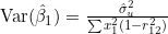
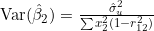

Where  is the correlation coefficient squared between X1 and X2. If it equals 1, the standard errors and covariance are infinite, and as collinearity increases, the variances and covariances of the two estimators also increase.
The speed with which variances and covariances of estimators increase is measured by the Variance Inflation Factor (VIF). It is calculated as:
If X-variables are perfectly correlated, then VIF approaches 0. If the correlation coefficient between X1 and X2 tends to 1, VIF becomes infinite. If X-variables are not correlated at all, then VIF=1.

The inverse of VIF is called Tolerance. It is calculated as:

If VIF increases, TOL will decrease.
Relationship between Correlation Coefficient, VIF, and Tolerance
 | VIF | TOL=1/VIF |
| 0 | 1 | 1 |
| 0.5 | 1.33 | 0.75 |
| 0.7 | 1.96 | 0.51 |
| 0.8 | 2.78 | 0.36 |
| 0.9 | 5.76 | 0.17 |
| 0.95 | 10.26 | 0.1 |
| 0.97 | 16.92 | 0.06 |
| 0.99 | 50.25 | 0.02 |
| 0.995 | 100 | 0.01 |
| 0.999 | 500 | 0 |
Wider Confidence Intervals
Multicollinearity leads to wider confidence intervals because it increases the standard errors of the estimated regression coefficients. The formula to calculate the confidence interval is:
![95\%\,CI \text{ for } \beta_i = \left[\hat{\beta}_i - t_{\alpha/2}\, \mathrm{se}(\hat{\beta}_i),\; \hat{\beta}_i + t_{\alpha/2}\, \mathrm{se}(\hat{\beta}_i)\right]](https://minhajmetrixhub.com/wp-content/ql-cache/quicklatex.com-0c1859843b8c417300e6b2539ffa364b_l3.png "Rendered by QuickLaTeX.com")
Wider confidence intervals lead to the acceptance of the null hypothesis very often, resulting in the insignificance of coefficients.
Insignificant “t-ratios”
Multicollinearity leads to “insignificant” t-ratios because it inflates the standard errors of the estimated coefficients, which reduces the value of the t-statistic. The t-ratio is calculated as the estimated coefficient divided by its standard error. This results in a failure to reject the null hypothesis, making the variable appear statistically insignificant, even though it may actually be important.

Causes/Sources of Multicollinearity
- Limited variability in data: When data is collected over a limited range of values, the variables may appear more closely related than they actually are.
- Constraints on the model or population being sampled: For example, in the regression of electricity consumption (Y) on income (X1) and house size (X2), there is a physical constraint in the population in that families with higher incomes generally have larger homes.
- Adding polynomial terms): Including polynomial terms (like X, X2, X3 ) or interaction terms (X1*X2) can create high correlation among regressors.
- Over-determined model: When the number of independent variables (k) exceeds the number of observations (n), it leads to multicollinearity. This situation is common in medical research.
- Common trends: Time series variables like GDP, population, and investment often have similar upward or downward trends over time, leading to multicollinearity.
- Dummy variable trap: When we introduce as many dummies as there are categories without excluding a base/reference category it leads to perfect multicollinearity.
- Different units or scales of measurement: Using the same variable in different units (e.g., price in PKR and USD) may cause collinearity.
- Inclusion of overlapping or closely related variables: For example, including both years of education and education level (primary, secondary, etc.) can cause multicollinearity.
- Including lagged terms: In time series data, using lagged values of variables (e.g.,
 ) may lead to multicollinearity if they are highly correlated with each other.
 ) may lead to multicollinearity if they are highly correlated with each other.
Detection of Multicollinearity
1. High R2 but few significant t-ratios
This is the “classic” symptom of multicollinearity. If R2 is high, say more than 0.8, and the F test suggests that the overall model is significant, but none or few individual t-ratios of regression coefficients are statistically significant than there might be multicollinearity.
2. High Pair-Wise Correlations among Regressors.
If the pairwise or zero-order correlation coefficient between two regressors is high, say, more than 0.8, then multicollinearity is a serious problem.
3. Examination of Partial Correlations
Farrar and Glauber have suggested examining partial correlation coefficients. Thus, in the regression of  , a finding that overall
  is very high but
  are comparatively low may suggest that the variables
  are highly intercorrelated.
4. Auxiliary Regression.
Another way to detect multicollinearity is to run auxiliary regression among explanatory variables and compute R2 from each regression, which we will call  . From each R2 we can compute the F value corresponding to each auxiliary regression from the following equation.
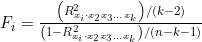
If the computed F exceeds the critical F at the chosen level of significance, we conclude that the particular Xi is collinear with other X’s; if it does not exceed the critical F, we say that it is not collinear with other X’s.
5. Klein Rule of Thumb.
The Kelin rule of thumb criterion states that if R2 obtained from an auxiliary regression is greater than the overall R2 this suggests multicollinearity.
6. Tolerance or Variance Inflation Factor.
The variance inflation factor shows how the variance of the estimator is inflated by the presence of multicollinearity. If the VIF value exceeds 10 it suggests that the variable is highly collinear and needs to be corrected. The closer TOLj is to zero, the greater the degree of collinearity of that variable with the other regressors.


7. Scatterplot
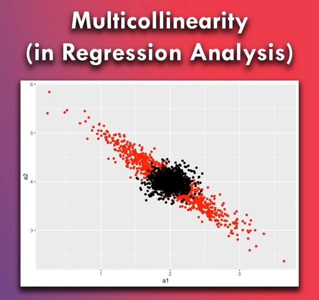
It is natural to see the scatter plot for the relationship among explanatory variables. If the scatterplot between two X variables is close to a straight line, it suggests that these two X variables are highly collinear.
8. Eigenvalues and Condition Index.
Using various software, we can find eigenvalues and the condition indices to diagnose multicollinearity. From eigenvalues, we can derive the condition number, k, and condition index, CI, by the following formula.


- = maximum eigenvalues
- = minimum eigenvalues
If k exceeds 1000 or CI exceeds 30, then there would be severe multicollinearity.
Remedial Measures for Multicollinearity
- Do nothing: Multicollinearity is a natural phenomenon, therefore no corrective measures are necessary. This is particularly true if the goal is prediction rather than inference.
- Use panel data to increase variability: Another approach used to reduce multicollinearity is to combine cross-sectional and time series data (panel data), which increases the variation in the dataset.
- Remove highly collinear variables: Dropping one or more variables with high Variance Inflation Factors (VIF > 10) can mitigate multicollinearity. However, this approach may lead to omitted variable bias or misspecification if important variables are removed.
- Transform the variables: In time series data, applying transformations such as logarithms, first differences, or growth rates can help eliminate trends and reduce multicollinearity.
- Increase the sample size: Adding more observations increases the variability in the data and can help reduce multicollinearity.
- Use dimensionality reduction techniques: Multivariate techniques like Factor Analysis and Principal Components Analysis (PCA) can be used to combine collinear variables.
- Apply regularisation methods: Techniques such as Ridge Regression and Lasso Regression introduce a penalty term to the regression estimates, shrinking the coefficients and helping to stabilise the model when multicollinearity is present.
Suggestions for further readings







 MinhajMetricsHub
2 responses to “Multicollinearity: Types, Concequences, Causes, Detection & Remedies”
[…] Multicollinearity: Types, Concequences, Causes, Detection & Remedies […]
[…] Multicollinearity: Types, Concequences, Causes, Detection & Remedies […]