

Saving Function
Definition
The saving function shows the functional relationship between saving and disposable income. It tells us how much a household wants to save at a given income level. Thus, S = f(Y).
Equation

Where C₀ = autonomous consumption, c = MPC
or

Where S₀ = −C₀ (autonomous saving/dissaving) s = 1 − c (MPS = 1 − MPC)
Autonomous Saving ‘S₀’
Autonomous saving is the part of saving that does not depend on current income and is represented by the intercept of the saving function. It is found when Y=0 in the saving function. S = S₀ + s Y When Y=0, S=S₀
Important Points
- Intercept of Saving Function: It is represented by the vertical intercept of the saving function when Y=0.
- Independent of Income: Autonomous saving does not depend on the current level of income. It remains constant even when income changes.
- Represents Dissaving: It is the amount households dissave (negative saving) or save when Y is zero.
Example: If S= -500+0.2Y, then -500 represent autonomous saving/dissaving
Induced Saving ‘sY’
Induced saving is that part of savings which depends on disposable income. It is found by multiplying MPS with disposable income. As income rises, people usually save more; as income falls, they save less. Induced Saving = MPS × Y
Important points
- Depends on Income: Varies directly with the level of income. As income increases, induced saving increases and vice versa.
- Zero at Zero Income: When income is zero, induced saving is also zero because it is generated by income.
- Depends on MPS: Higher MPS means people save more out of their income.
Example: If S=-500+0.2Y, when Y=1000, sY=200
Marginal Propensity to Save (MPS)
Definition
MPS (Marginal Propensity to Save) is the change in saving (ΔS) resulting from a one-unit change in disposable income (ΔY). MPS = ΔS / ΔY
Important Points
- Slope of Saving Curve: MPS is the slope of the saving function. A steeper saving curve → higher MPS.
- Relationship to MPC: If MPC = 0.8 then MPS = 0.2. Every income rupee is either consumed or saved.
Example: If income rises by  20 → MPS = 20/100 = 0.2
Average Propensity to Save (APS)
Definition
APS (Average Propensity to Save) is the fraction of total disposable income that is saved at a given income level. APS = S / Y
Properties of APS:
- APS = 1 − APC (derived from Y = C + S)
- APS rises as income rises (saving rate ↑)
- APS can be negative at low incomes (dissaving)
Relationship to APC: APC + APS = 1. If APC = 0.8 then APS = 0.2. Income is either consumed or saved.
Note: APC + APS = 1 and MPC + MPS = 1 (fundamental identities)
Relation B/W MPC & MPS
National income identity

Take changes on both sides

Divide both sides by ΔY

Simplify

Use definitions of MPC and MPS

Final Relationship

If we have to find MPC or MPS we can use the following formulas:
MPC = 1 – MPS or MPS = 1 − MPC
Example: If MPC=0.8, then MPS=1-MPC=1-0.8=0.2
Relation B/W APC & APS
National income identity
Take changes on both sides

Simplify

Use the definitions of APC and APS

Final Relationship

If we have to find APC na dAPS we can use the following formulas:
APC = 1 – APS or APS = 1 − APC
Example: If APC=0.6, then APS=1-APC=1-0.6=0.4
Derivation of Saving Function
Mathematical Derivation
Start with the consumption function

National income identity
Rearrange for saving

Substitute the consumption function

Expand the bracket

Rearrange and collect terms
Final Equation

Tabular Derivation
| Income (Y) | Consumption (C) | Saving (S = Y − C) | APC = C/Y | MPC = ΔC/ΔY | APS = 1 − APC | MPS = 1 − MPC |
| 0 | 40 | −40 | — | — | — | — |
| 100 | 120 | −20 | 1.2 | 0.8 | −0.20 | 0.2 |
| 200 | 200 | 0 | 1 | 0.8 | 0 | 0.2 |
| 300 | 280 | 20 | 0.93 | 0.8 | 0.07 | 0.2 |
| 400 | 360 | 40 | 0.9 | 0.8 | 0.1 | 0.2 |
| 500 | 440 | 60 | 0.88 | 0.8 | 0.12 | 0.2 |
| 600 | 520 | 80 | 0.87 | 0.8 | 0.13 | 0.2 |
Graphical Derivation
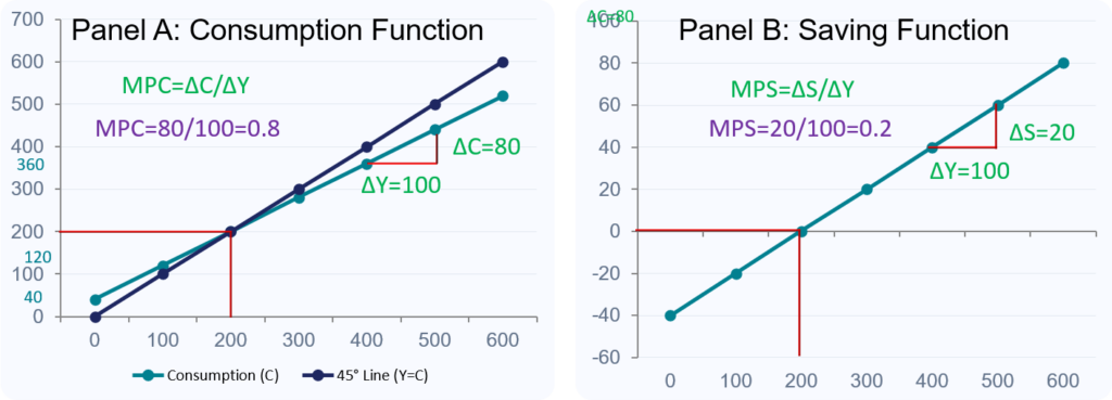
The saving curve SS is the vertical gap between the 45° line and consumption curve CC. Before Y = 200 there is dissaving; at Y = 200 saving is zero (break-even); beyond Y = 200 saving is positive and rising.
Suggestions for further readings






 MinhajMetricsHub