Simple Linear Regression Model

Table of Contents

Simple Linear Regression Model

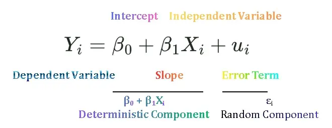
Simple Linear Regression Model is used to estimate the relationship between one dependent and one independent variable. It is also called bivariate or two variable regression model. For example, regression of consumption on disposable income, regression of sales revenue on advertisement expenses, regression of log of wages on years of education. In previous we discussed the concepts of population and sample regression function. To access previous lecture click here Population Regression Function and Sample Regression Function.

Least Square Principle

We found out primary objective to estimate PRF.

$Y_i = \beta_0 + \beta_1 X_i + u_i$ … 1

on the basis of the SRF

${ Y}_i = \hat{\beta}_0 + \hat{\beta}_1 X_i + \hat{u}_i$ … 2

We cannot estimate the PRF accurately because of sampling fluctuations. Therefore, given a sample, we approximate the true relationship by estimating the SRF. But how the SRF itself is estimated from the sample? This is the main focus of this post.

We want to derive SRF such that it is as close as possible to the actual or observed values of Y. It can be done if we choose SRF in such a manner that the difference between actual Y and estimated Y is as small as possible. We have various criterions to minimize this distance. These are:

Minimize the sum of errors i.e. $\sum e_i$
Minimise the absolute sum of errors i.e. $\sum |e_i|$
Minimise the weighted sum of absolute errors i.e. $\sum w_i |e_i|$

Minimize the sum of residuals i.e. $\sum e_i$

Minimizing the sum of residuals is not a good criterion because of two reasons. Firstly, sum of residuals are zero because positive and negative errors cancel out each other or too small even though errors are widely spread around the regression line. If we minimise sum of residuals this would be misleading. Secondly, each error gets equal weight in the sum $(u_1 + u_2 + u_3 + u_4)$ though large or small. In other words, large and small errors have equal importance and are treated as same.

e_i	Case A	Case B	Case C	Case D
e₁	500	0	0	\|14\|
e₂	-900	10	0	\|-14\|
e₃	-500	0	50	14\|
e₄	900	0	0	\|-14\|
Sum of e_i	0	10	50	56

In table 1 case B is more desirable than case A, although it has non-zero sum, but error is small but in case A although sum of residuals is zero, but the errors are large.

Minimise the absolute sum of residuals i.e. $\sum |e_i|$

The second option we have is to take the absolute sum of residuals so that the sum of residuals cannot be zero. There is another problem in this method, that it ignores outliers. Suppose that in case C we have one outlier while other errors are zero. If we fit the line, the fit might not be as good because it ignores the outlier. In case D we have relatively large errors in absolute terms, but we might like case D because it considers all the errors value, but still, it has a problem of equal weights.

Minimise the weighted sum of absolute residuals i.e. $\sum w_i |e_i|$

The third option we have is to minimize the sum of squared residuals to give more importance to large errors and less importance to small errors and then minimize the errors. Let w_i =|e_i|

$\sum w_i |e_i|$

$\sum |e_i| \, |e_i|$

$\sum (|e_i|)^2$

$\sum e_i^2$

This is the basis of the Ordinary Least Square Method. So, minimizing the squared residuals has several advantages over either minimizing sum of residuals or minimizing sum of absolute residuals. Firstly, the sum of squared residuals is not always zero and, secondly, it gives more importance to large errors and little importance to small errors. A further justification for the least-squares method lies in the fact that the estimators obtained by it have some very desirable statistical properties, as we shall see later.

Least square principle is the mathematical procedure that uses the data to position a line with the objective of minimizing sum of the squared vertical distance between the actual Y values and the predicted values of Y.

In other words, least square method chooses the $\hat{\beta}_0$ and $\hat{\beta}_1$ in such a manner that in a given set of data $\sum e_i^2$ is as small as possible.

Derivation of OLS

Consider a two-variable population regression model

$Y_i = \beta_0 + \beta_1 X_i + u_i$

which we estimate using SRF

$\hat{Y}_i = \hat{\beta}_0 + \hat{\beta}_1 X_i$

Residuals are given as:

$\hat{u}_i = Y_i - \hat{Y}_i$

$\hat{u}_i = Y_i - \hat{\beta}_0 - \hat{\beta}_1 X_i$

Squaring the residuals

$SSR = \sum_{i=1}^{n} \hat{u}_i^2$

$SSR = \sum_{i=1}^{n} (Y_i - \hat{\beta}_0 - \hat{\beta}_1 X_i)^2$ … (1)

Take partial derivative of equation 1 w.r.t $\hat{\beta}_0$ and set it equal to zero

$\frac{\partial SSR}{\partial \hat{\beta}_0} = -2 \sum_{i=1}^{n} (Y_i - \hat{\beta}_0 - \hat{\beta}_1 X_i) = 0$

$\sum_{i=1}^{n} Y_i = n \hat{\beta}_0 + \hat{\beta}_1 \sum_{i=1}^{n} X_i$ … (2)

Now take partial derivative of equation 1 w.r.t $\hat{\beta}_1$ and set it equal to zero

$\frac{\partial SSR}{\partial \hat{\beta}_1} = -2 \sum_{i=1}^{n} X_i (Y_i - \hat{\beta}_0 - \hat{\beta}_1 X_i) = 0$

$\sum_{i=1}^{n} X_i Y_i = \hat{\beta}_0 \sum_{i=1}^{n} X_i + \hat{\beta}_1 \sum_{i=1}^{n} X_i^2$ … (3)

Solving equations (2) and (3) simultaneously we get formulas of $\hat{\beta}_0$ and $\hat{\beta}_1$

$\hat{\beta}_1 = \frac{\sum_{i=1}^{n} (X_i - \bar{X})(Y_i - \bar{Y})}{\sum_{i=1}^{n} (X_i - \bar{X})^2}$

$\hat{\beta}_0 = \bar{Y} - \hat{\beta}_1 \bar{X}$

Numerical Properties of OLS Estimators

Numerical properties are those that hold as a result of the use of ordinary least squares, regardless of how the data were generated. These properties are:

The OLS estimators are expressed solely in terms of the observable (i.e., sample) quantities (i.e., X and Y). Thus, we have given the data of X and Y we can easily estimate the values of $\hat{\beta}_0$ and $\hat{\beta}_1$ .
OLS estimators are point estimator, it means they provide only a single value of population parameter. Interval estimators are those which provide a range of values for population parameter.
Once the OLS estimates are obtained, we can easily draw sample regression line. This sample line has the following five properties.

1. It passes through the sample means of Y and X. It can be seen from the following equation.

$\hat{\beta}_0 = \bar{Y} - \hat{\beta}_1 \bar{X}$

2. The mean value of the estimated $\hat{Y}_i$ is equal to the mean value of the actual Y. That is.

$\bar{\hat{Y}} = \bar{Y}$

3. The mean value of the residuals $Y = \hat{Y}_i$ is zero.

$E(\hat{u}_i) = 0$

4. The residuals $Y = \hat{Y}_i$ are uncorrelated with the predicted Y.

$\operatorname{Cov}(\hat{Y}_i, \hat{u}_i) = 0$

5. The residuals $Y = \hat{Y}_i$ are uncorrelated with X.

$\operatorname{Cov}(X_i, \hat{u}_i) = 0$

Statistical Properties of OLS Estimators

The statistical properties of OLS estimators are those that hold only under certain assumptions about the way the data were generated. Statistical properties of OLS estimators are of two categories:

Finite or small sample properties (properties that hold regardless of the sample size under certain assumptions known as Gauss-Markow assumptions): These properties include unbiasedness, minimum variance and efficiency.
Asymptotic or large sample properties (properties that hold only if the sample size is very large (technically, infinite): These properties include consistency, asymptotic unbiasedness, asymptotic efficiency. asymptotic normality.

Some Concepts

Conditional Mean

The conditional mean in regression analysis is the expected value of the dependent variable Y given a specific value of the independent variable (X), denote as E (Y| X_i) It is expressed as the function of value of X, X_i written as E (Y| X_i) = f(X_i)

Stochastic Error Term

Stochastic error term of error term is PRF shows the difference between actual or observed value of Y and conditional mean value of Y. That is, $u_i = Y_i - E(Y \mid X_i)$ . In other words it represents the vertical distance between each value of Y and its conditional mean. Error term can be positive or negative. It is positive when Y>E(Y|Xi). It is negative when Y<E(Y|Xi). It is zero when Y=E(Y|Xi). Thus, Y fluctuates around E(Y|Xi). Why? It is because there are lot of unobserved factors that affect Y but cannot be included in our model. These are omitted factors and error term captures their collective effect.

Error vs Residual

Error (µ) is the error of specification. It can be controlled if we choose a good model or we able to extract as much information from µ. Residual (e) is the error of estimation. It is inevitable. In OLS our task is to minimise the estimation error.

Interpretation of Simple Linear Regression Estimates

After estimating simple linear regression coefficients, it is important to interpret its results. Remember that in SLRM a dependent variable is expressed as the linear function of only on independent variable. The slope coefficient in SLRM measures the change in Y due to one unit change in X. In other words, slope coefficient tells us if X increases by one unit, then by how much Y will increase or decrease depending on the sign of the coefficient. Or the slope $\hat{\beta}_1$ means that, for each increase of one unit in X, the mean value of Y i.e., $\hat{Y}$ , changes by the magnitude of $\hat{\beta}_1$ units. The interpretation of slope coefficient depends on the units of dependent and independent variables in which they are measured. Consider couple of examples:

Suppose Y=Per house cost in USD, X= house size in square foot. $\hat{\beta}_1$ =75, it means for each one square ft. increase in house size increases its cost by USD 75.
Consider another example, Y=quantity consumed in kg, X=price in PKR. $\hat{\beta}_1$ =2.716, it means that for each one PKR increase in price, quantity consumed will fall by 2.716 kg.

Now consider the interpretation of intercept also known as constant, $\hat{\beta}_0$ . It is the mean of dependent variable when X=0. If $\hat{\beta}_0$ =25000, it means that

Suggestions for Further readings:

Share this article

Muhammad Minhaj Akhtar

Muhammad Minhaj Akhtar is a Lecturer in Economics at Government Graduate College Jauharabad, Pakistan. He holds an M.Phil. in Economics from Quaid-i-Azam University, Islamabad, and an MSc in Economics from the University of Sargodha, where he earned a Silver Medal. His academic passion lies in Econometrics, with a strong focus on applying empirical methods to real-world economic issues. Through MinhajMetrixHub, he shares learning resources, research guidance, and practical econometric insights for students and researchers.

Read Posts

Simple Linear Regression Model

Simple Linear Regression Model

Least Square Principle

Derivation of OLS

Numerical Properties of OLS Estimators

Statistical Properties of OLS Estimators

Error vs Residual

Interpretation of Simple Linear Regression Estimates

Share this article

Muhammad Minhaj Akhtar

Leave a Reply Cancel reply

CATEGORIES

TAGS

Recent Posts

Microeconomic Household Fertility Theory

Inflation, Its Types, Causes and Effects

Malthus Population Theory

Nominal GDP, Real GDP & GDP Deflator

Solow Model of Economic Growth