Regression Through Origin

Introduction of Regression Through Origin Models

So far we have studied models like

Where intercept is present. An economic example of these models is the Keynes consumption function written as:

Where  is autonomous consumption i.e., level of consumption when income is zero.

In some cases, we wish to impose the restriction that, when x=0, the expected value of y is zero. There are certain relationships for which this is reasonable. For example, in the following model where tax revenue depends on income:

If income (X) is zero, then income tax revenues (Y) must also be zero.

Consider another example from production theory:

If output is zero (X=0), the variable cost will also be zero (Y=0).

Definition of Regression Through Origin Models

A regression model in which intercept term ( ) is absent or zero is called regression through origin model because it passes through the origin i.e., where X=0, and Y=0. It can be written as:

Economic Examples of Regression Through Origin Models

Instances where the zero-intercept model may be appropriate are

• Milton Friedman’s permanent income hypothesis, which states that permanent consumption  is proportional to permanent income, , that is . 
• Cost theory which postulates that the variable cost of production is proportional to output.
• Some versions of monetary theory which state that the rate of change of prices (i.e., the rate of inflation) is proportional to the rate of change of the money supply.

Estimation of Regression Through Origin Models

Corresponding to equation 1 we can write our sample regression function as.

Or

To obtain the slope coefficient, we still rely on the method of ordinary least squares, which in this case minimizes the sum of squared residuals.

And

It is interesting to compare these formulas with those obtained when the intercept term is included in the model.

Difference between Intercept and without Intercept Models

1. In the model with no intercept, we use raw sums of squares and cross products but in the model with intercept, we use deviations from mean sums of squares and cross products.
2. The degrees of freedom in model with intercept to estimate the variance of residual is n-2, but df in the model without intercept is n-1.
3. The r², the coefficient of determination is always non-negative for the conventional model, but for interceptless model it can turn out to be negative! This anomalous result arises because the r² explicitly assumes that the intercept is included in the model.

Consequences of using Zero Intercept Models.

1. In models with intercept sum of residuals is always zero but in models without intercept zero mean of residual is not necessary. Thus, we must use the interceptless models only when it is appropriate.
2. If we omit the constant term, then the impact of the constant is forced into the estimates of the other coefficients, causing potential bias.

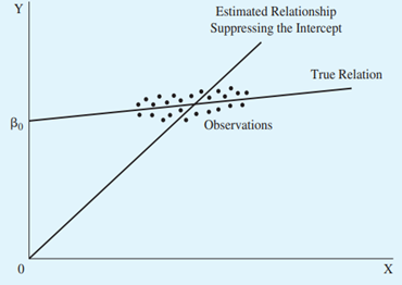
Example:

Suppose we run a regression model both with and without intercept. Estimating a regression equation with a constant term would likely produce an estimated regression line very similar to the true regression line, which has a constant term quite different from zero. The slope of this estimated line is very low, and the t-score of the estimated slope coefficient may be very close to zero.

However, if the researcher estimates the model without intercept, which implies that the estimated regression line must pass through the origin, then the estimated regression line would result the slope coefficient is biased upward compared with the true slope coefficient. The t-score is biased upward as well, and it may indicate that the estimated slope coefficient is significantly positive. Such a conclusion would be incorrect.

Regression with and without intercept.

Coefficient of Determination for Regression Through Origin Model.

To calculate r² for models without intercept we can use the following formula.

Note that here cross products and sum of squares are in raw form i.e., not mean corrected that`s why we call r² of regression through origin as raw r².

Although this raw r² satisfies the relation 0 < r² < 1, it is not directly comparable to the conventional r² value. For this reason, some authors do not report the r² value for zero intercept regression models.

Conclusion

Because of these special features of this model, we need great caution in using the zero-intercept regression model. Unless there is a very priori expectation, one would be advised to use the conventional, intercept-present model. This has a dual advantage.

• First, if the intercept term is included in the model but it turns out to be statistically insignificant (i.e., statistically equal to zero), for all practical purposes we have a regression through the origin.
• Second, and more important, if in fact there is an intercept in the model, but we insist on fitting a regression through the origin, we would be committing a specification error.