
In the previous article, Assumptions of Classical Linear Regression Model (CLRM), we discussed the assumptions of CLRM. In this article, we discuss the variance and standard error of OLS estimators and the Gauss-Markov Theorem.
It has been shown in the post Simple Linear Regression Model that the OLS estimates are a function of sample values of X and Y. But since the data are likely to change from sample to sample (X is fixed in repeated sampling), the estimates will also change from sample to sample. How much will our sample estimates change if we repeat the hypothetical process of repeated sampling? In other words, how accurate or precise are our sample estimates?
This accuracy and precision of OLS estimates can be measured by their standard error. Given the Gaussian assumptions as discussed in the post Assumptions of Classical Linear Regression Model (CLRM), the variance and standard error of OLS estimates can be obtained as follows:
Variance and Standard Error of OLS Estimators
Variance of 

Standard error of

Variance of 

Standard error of

where var = variance and se = standard error, and where σ2 is the constant or homoscedastic variance of ui, which is unknown since the population is unknown; therefore, we estimate it using  , which itself can be found using the following formula:

Where is the OLS estimator of the true but unknown  , and where the expression n − 2 is known as the number of degrees of freedom (df),
  is the residual sum of squares (RSS).
Once is known, can be easily computed. itself can be computed either from  or from the following expression:


Features of Variance and Standard Error of OLS Estimators
 but inversely proportional to
  . That is, given σ2, the larger the variation in the X values, the smaller the variance of
  but inversely proportional to

Since var () is always positive. The nature of the covariance between and depends on the sign of  . If
. If  is positive, then as the formula shows, the covariance will be negative.
Thus, if the slope coefficient β1 is overestimated (i.e., the slope is too steep), the intercept coefficient β0 will be underestimated (i.e., the intercept will be too small).
Gauss-Markov Theorem (Finite Sample Properties of OLS Estimators)
Given the assumptions of the classical linear regression model (CLRM), the OLS estimators have the minimum variance among the class of all linear unbiased estimators; that is, they are the best linear unbiased estimators (BLUE).
The best linear unbiased property of OLS estimators is explained below.
 and are Linear estimators; that is, they are linear functions of the random variable Y.
- They are Unbiased, that is,
 . Therefore, in repeated applications, on average and will converge with their true values
  and , respectively.
 - They are Best, that is they have minimum variance in the class of all linear unbiased estimators.
 . Therefore, in repeated applications, on average
  and
and Sampling Distribution of OLS Estimators
The sampling distribution of an estimator is simply a probability or frequency distribution of the estimator, that is, a distribution of the set of values of the estimator obtained from all possible samples of the same size from a given population. Sampling distributions are used to draw inferences about the values of the population parameters on the basis of the values of the estimators calculated from one or more samples.
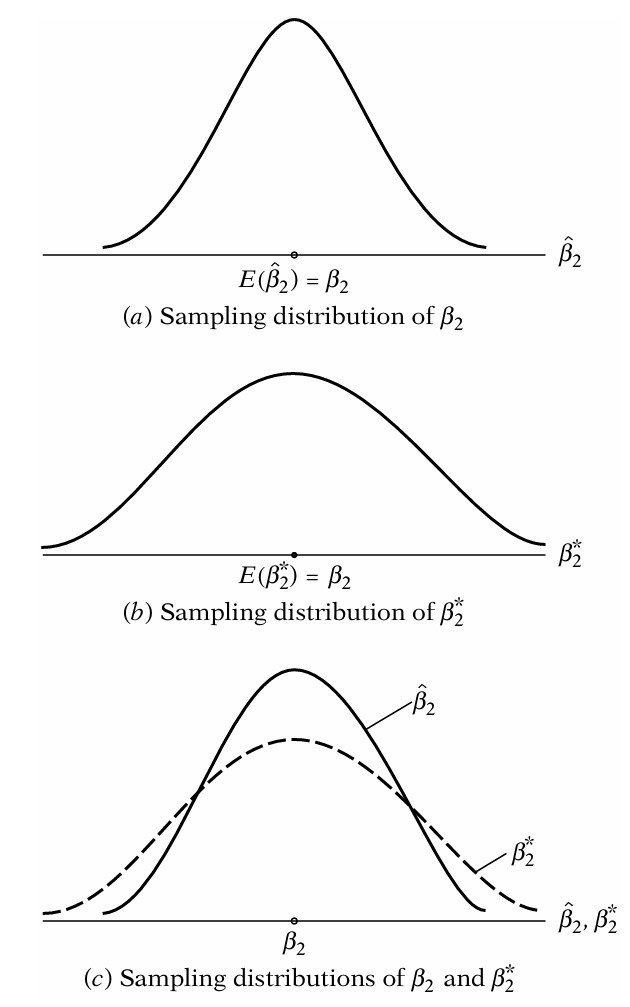
The sampling distribution of the OLS estimator is the distribution of the values taken by in repeated sampling experiments. Suppose that we take 100 random samples from a given population of the same size ‘n’, its probability distribution is shown in Figure 1(a).
If we assume that the is distributed symmetrically, as shown, the mean or expected value of is equal to  . This is the unbiasedness property of . Thus, is the unbiased estimator of . An estimator is said to be unbiased if its expected or mean value is equal to its true parameter, that is
  .
.
In Figure 1(b), we show the sampling distribution of  . It is an alternative estimator of obtained by using another (i.e., other than OLS) method. Assume that like is unbiased and linear. Which estimator should we rely on?
To answer this question, we have combined both parts of Figure 1 in Figure 1(c). You can observe that is more widely spread around the mean value than the distribution of . In other words, the variance of is larger than the variance of , that is,  .
.
Thus, we can say that though both and are linear and unbiased estimators of , is more efficient than , since the former has smaller variance. Therefore, is the best estimator of . An estimator is said to be best if it has minimum variance among all linear unbiased estimators.
Some Concepts
Expected Value of OLS Estimator
The expected value of the OLS estimator is the mean value of the estimator in its sampling distribution.
Standard Error
Standard error is the standard deviation of the sampling distribution of the estimator.
Linear Estimator
An estimator is said to be linear if it can be expressed as a linear function of the dependent variable, Y
Unbiased Estimator
An estimator is said to be unbiased if its expected or mean value is equal to its true parameter, that is .
Best Estimator
An estimator is said to be best if it has minimum variance among all linear unbiased estimators.
Efficient Estimator
An estimator is said to be efficient if it has minimum variance among all unbased estimators.
Finite Sample Properties of OLS Estimators
The BLUE (Best Linear Unbiased Estimator) property of OLS is a finite sample property of OLS estimator. BLUE property of the OLS estimator holds as long as the Gauss-Markov assumptions hold.
Asymptotic Properties of OLS Estimators
Asymptotic properties are the properties that hold only if the sample size is very large (technically, infinite). These properties are consistency, asymptotic unbiasedness, asymptotic normality, and asymptotic efficiency.


 MinhajMetricsHub