Assumptions of Classical Linear Regression Model (CLRM)

In the previous post, we discussed how to estimate a sample regression model, i.e., $\hat{\beta}_0$ and $\hat{\beta}_1$ . by applying the OLS method on sample data, both in simple and multiple linear regression models. You can read these posts here: A Numerical Example of Multiple Linear Regression by Hand and Simple Linear Regression Model.

But our purpose is not only to estimate the sample estimates $\hat{\beta}_0$ and $\hat{\beta}_1$ . but also to draw inferences about the true population parameters (β₁ and β₂).. In other words, we want to know how close $\hat{\beta}_0$ and $\hat{\beta}_1$ are to their population counterparts, β₁ and β₂. Or how close $\hat{Y}_i$ is it to the true E(Y | Xi). That is, we must know how good our sample estimates $\hat{\beta}_0$ and $\hat{\beta}_1$ are.

We can prove that OLS estimates are best under certain assumptions. These assumptions are called ‘classical assumptions’. We will see in the next blogs that OLS estimators are the best linear unbiased estimators (BLUE) of true population parameters when these classical assumptions are met, known as the Gauss-Markov theorem, which states that

Given the assumptions of the classical linear regression model, the least-squares estimators, in the class of all linear unbiased estimators, have minimum variance, that is, they are BLUE.

Since in PRF Y_i not only depends on Xi but also on u_i.Therefore, we must have knowledge of how X_i and u_i are generated, which requires some assumptions about them. Below, we discuss assumptions related to X_i and u_i.

Table of Contents

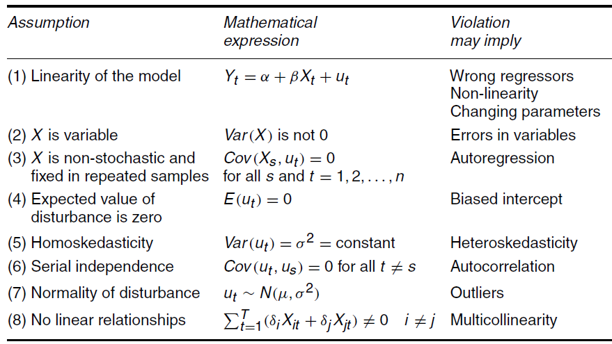
Assumptions of Classical Linear Regression Model

A1: Linear Regression Model

The regression model is linear in parameters, though it may be linear or nonlinear in the variables. A regression model is said to be linear in parameters if $\beta$ appears with a power of 1 only and not in terms like $\beta^2$ , $\beta_1 \beta_2$ , $\frac{\beta_1}{\beta_2}$ , $\sqrt{\beta}$ , $X^{\beta}$ etc. Here are some examples:

$Y_i = \beta_0 + \beta_1 X_i^2$ Nonlinear in variables but linear in parameters

$Y_i = \beta_0 + \beta_1^2 X_i$ Linear in variables but nonlinear in parameters

$Y_i = \beta_0 + \beta_1 X_i$ Linear in variables as well as parameters

$Y_i = \beta_0 + \beta_1^2 X_i^2$ Nonlinear in parameters as well as nonlinear in variables

Two meanings of linearity:

Linearity in Variables

Linearity in variables can be defined in two alternative ways:

Linearity in terms of power of X: The function Y is said to be linear with respect to X if X appears with a power of 1 only. For example, if $Y_i = \beta_0 + \beta_1 X_i + u_i$ , this model is said to be linear in variables, since X appears with power 1 only. The model $Y_i = \beta_0 + \beta_1 X_i^2 + u_i$ is said to be a non-linear function because $X$ appears in squared form. Similarly, if X appears in forms like $\sqrt{X}$ , $X \cdot Z$ , $\frac{X}{Z}$ , $e^{X}$ , $\frac{1}{X}$ , the function is said to be non-linear.
Linearity in terms of slope coefficient: Another way of expressing the linearity in the variables is that the slope of Y with respect to X, i.e., the rate of change of Y with respect to X (dY/dX) must be independent of the variable X. For the model like $Y_i = \beta_0 + \beta_1 X_i + u_i$ , the slope is $\beta_1$ . But for a model like $Y_i = \beta_0 + \beta_1 X_i^2 + u_i$ , the slope would be $\beta_1 \cdot 2X$ , where the slope $\beta_1$ depends on variable X.

Linearity in Parameters

Linearity in parameters can be defined in two alternative ways:

Linearity w.r.t. power of parameter: A regression model is said to be linear in parameters if $\beta$ appears with a power of 1 only and not in terms like $\beta^2$ , $\beta_1 \beta_2$ , $\frac{\beta_1}{\beta_2}$ , $\sqrt{\beta}$ , $X^{\beta}$ etc Therefore a model $Y_i = \beta_0 + \beta_1 X_i^2 + e_i$ is linear in parameters since all parameters appear with the power of 1. But the model $Y_i = \beta_0 + \beta_1^2 X_i + e_i$ , is said to be non-inear in parameters.since $\beta_1$ apears in square form.
Linearity w.r.t. partial derivative: Another way of expressing the linearity is that, if all the partial derivatives of Y with respect to each of the parameters i.e., $\beta_1, \beta_2, \beta_3, \ldots$ etc., are independent of the parameters, then the model is called a linear model. For example, if the model is $Y_i = \beta_0 + \beta_1 X_{1i}^2 + \beta_2 \sqrt{X_{2i}} + \beta_3 \log(X_{3i}) + e_i$ and we take partial derivative of Y w.r.t. $\beta_1$ , it would be $\frac{\partial Y}{\partial \beta_1} = X_1^2$ . But if the model is $Y_i = \beta_0 + \beta_1^2 X_{1i}^2 + \beta_2 \sqrt{X_{2i}} + \beta_3 \log(X_{3i}) + e_i$ , its partial derivative w.r.t. $\beta_1$ would be $\frac{\partial Y}{\partial \beta_1} = 2 \beta_1 X_1^2$ , which depends on parameter $\beta_1$ . Thus, it is a non-linear (in parameters) model.

A2: Fixed X Values or X Values Independent of the Error Term

This assumption has two parts:

Values taken by the independent variable(s) are fixed in repeated sampling. It means if we repeat the sample multiple times, then in each sample, X values must be fixed while Y values may change since Y is a random variable.
If the regressors are stochastic, we assume that each regressor is uncorrelated with the error term. If X_i is correlated with the error term, endogeneity occurs, in which case estimates are biased and inconsistent.

What does it mean that X is fixed in repeated sampling? To understand this, consider the data on weekly consumption and weekly income measured in USD of 60 families in Table 1, which represents the population.

Table 1: Population data of 60 families

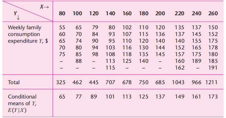
We take two random samples as shown in Table 2, and you can observe that in each sample, X values are fixed, while Y values can vary in each sample. For example, holding the value of income fixed at USD 80, we draw a family at random and observe that its weekly family consumption is USD 60. Still keeping X at USD 80, we draw at random another family and observe its Y value at USD 75. In each of these repeated samples, the value of X is fixed at USD 80. We can repeat this process for all the X values in both samples; in each case, X is fixed, but Y can vary.

Table 2: Random samples of 60 families

Sample 1		Sample 2
Y	X	Y	X
70	80	55	80
65	100	88	100
90	120	90	120
95	140	80	140
110	160	118	160
115	180	120	180
120	200	145	200
140	220	135	220
155	240	145	240
150	260	175	260

Now the question is, why do we assume that the X values are nonstochastic? Even though in most cases in social sciences, data are usually collected randomly on both the Y and X variables. It is due to the following reasons.

To simplify the analysis.
In most experimental studies, X is treated as fixed because it is controlled by the researcher, which helps in identifying cause-and-effect relationships. For example, a farmer divides his land into different parcels and applies different amounts of fertilizer to each parcel. In this experiment, the farmer has full control over the amount of fertiliser. By varying the amount of fertiliser, he can identify its effect on crop yield.
Even though we consider the case of stochastic regressors, the statistical results of linear regression found in the case of fixed regressors are also valid when the X’s are random, provided that some conditions are met. One condition is that regressor X and the error term ui are independent of each other.

Here, it is important to distinguish between the classical linear regression model (CLRM), where the regressors are assumed to be fixed, and the neoclassical regression model (NLRM), where the regressors are considered to be stochastic. In the former case, the model is called a fixed regressor model, and in the latter case, it is called a stochastic regressor model.

A3: Zero Mean Value of Disturbance u_i

Given the value of Xi, the mean, or expected value, of the random disturbance term u_i is zero. Symbolically,

$E(u_i \mid X_i) = 0$

Or, if X is non-stochastic,

$E(u_i) = 0$

This assumption means that the average or mean value of deviations around the regression line corresponding to any given X should be zero. This assumption simply means that the factors not explicitly included in the model, and therefore subsumed in ui, do not systematically affect the mean value of Y; in other words, the positive u_i values cancel out the negative u_i values so that their average or mean effect on Y is zero

This assumption implies that the model is correctly specified, i.e., there is no specification error or specification bias, which occurs when

We exclude important explanatory variables.
Including redundant variables.
Choose the wrong functional form.

It is important to note that if the conditional mean of one random variable given another random variable is zero, the covariance between the two variables is zero, and hence the two variables are uncorrelated. Assumption 3 therefore, implies that X_i and u_i are uncorrelated.

The reason for assuming that the disturbance term u and the explanatory variable(s) X are uncorrelated is that, when we write our PRF as $Y_i = \beta_0 + \beta_1 X_i + u_i$ we assume that u and X both have separate additive effects on Y. But when u is correlated with X, it is not possible to assess their individual effects on Y. In situations like this, it is quite possible that the error term actually includes some variables that should have been included as additional regressors in the model. Therefore, our model may be incorrectly specified.

A4: Homoscedasticity or Constant Variance of u_i

The word ‘homoscedasticity’ is derived from two Greek words: Homo, which means equal or same, and skedasticity, which means variance or spread or scatter. Thus, homoscedasticity means that the variance of the error term is constant for each value of X_i. Symbolically,

$\operatorname{Var}(u_i \mid X_i) = E(u_i^2 \mid X_i) = \sigma^2$

This assumption simply means that the variation around the regression line is the same across all values of X_i. i.e., the variance of u_i neither increases nor decreases, as X_i varies. That is, there will be the same distance between observed data points ( $Y_i$ ) and the regression line ( $\hat{Y}_i$ ). If this assumption is violated, it is called heteroscedasticity, which means that error variance is not the same across all values of X. It is written as

$\operatorname{Var}(u_i \mid X_i) = E(u_i^2 \mid X_i) = \sigma^2_i$

Proof

The variance of a random error term is given as

$\operatorname{Var}(u_i \mid X_i) = E\big[(u_i - E(u_i \mid X_i))^2\big]$

$E\big[u_i^2 - 2u_i E(u_i \mid X_i) + (E(u_i \mid X_i))^2\big]$

Given A3, the expected or mean value of u_i is 0, that is, $E(u_i \mid X_i) = 0$

$\operatorname{Var}(u_i \mid X_i) = E(u_i^2 \mid X_i) = \sigma^2$

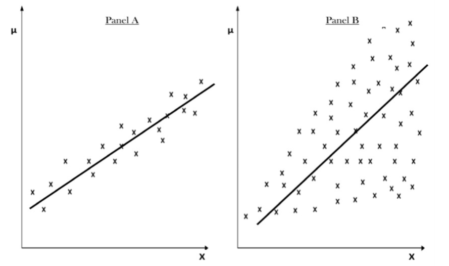
For instance, assume that Y is weekly consumption and X is weekly income of households. According to economic theory, we know that as income increases, family consumption expenditures also increase. The assumption of homoscedasticity states that the variance of consumption expenditure remains constant across all income levels. In other words, richer families on average consume more than poorer families, but there is also more variability in the consumption expenditure of the former. The cases of homoscedasticity (Panel A) and heteroscedasticity (Panel B)are shown in Figure 1.

Figure 1: Homoscedasticity and Heteroscedasticity

A5: No Autocorrelation between Disturbances:

The random error terms for different values of Xi, say u_i and u_j are independent, i.e., there is no correlation or covariance between the error terms of two different observations. In short, the observations are sampled independently. Symbolically,

$\operatorname{Cov}(u_i, u_j \mid X_i, X_j) = E(u_i u_j) = 0 \quad \text{for } i \neq j$

Since

$\operatorname{Cov}(u_i, u_j \mid X_i, X_j) = E\big[(u_i - E(u_i \mid X_i))(u_j - E(u_j \mid X_j))\big]$

Given A3, the expected or mean value of u_i and u_j are 0, that is, $E(u_i \mid X_i) = 0$ and $E(u_j \mid X_j) = 0$

$\operatorname{Cov}(u_i, u_j \mid X_i, X_j) = E\big[\, E(u_i \mid X_i)\, E(u_j \mid X_j)\,\big]$

In the absence of autocorrelation, the above Equation becomes zero.

$\operatorname{Cov}(u_i, u_j \mid X_i, X_j) = 0 \quad \text{for } i \neq j$

However, if there is correlation or covariance between the successive error terms for different values of Xi_, it implies ‘Autocorrelation’ or ‘Serial correlation.’ In the presence of autocorrelation, the covariance between u_i and u_jis not zero; it may be positive or negative depending on the type of correlation between error terms.

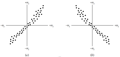
In case a positive ‘u’ is followed by a positive ‘u’ and a negative ‘u’ is followed by a negative ‘u’, it is a case of Positive autocorrelation. On the other hand, if a positive ‘u’ is followed by a negative ‘u’ and a negative ‘u’ is followed by a positive ‘u’, it is a case of Negative autocorrelation.

This problem of autocorrelation is usually associated with time series data, where the value of a variable at one point in time is often related to its values at previous points in time. Since time series data follow a natural ordering over time.

Figure 2: Positive and Negative Autocorrelation

A6: Number of Observations > Number of Parameters to Be Estimated:

The number of observations must be greater than the number of explanatory variables or parameters to be estimated. If for example, we have only one observation and two parameters, then we will be unable to estimate these parameters.

A7: Variability in X values:

This means that there should be some variation among the observations of the X variable, i.e., the observations of X variable must not be the same. Technically, Var (X) must be a positive number. This is because, if all the observations of X variable are the same, then

$X_i = \bar{X}$ therefore $\sum (X_i - \bar{X}) = 0$

If this is the case, it is impossible to compute $\hat{\beta}_1$ and $\hat{\beta}_0$

since

$\hat{\beta}_1 = \frac{\sum_{i=1}^{n} (X_i - \bar{X})(Y_i - \bar{Y})}{\sum_{i=1}^{n} (X_i - \bar{X})^2}$

$\hat{\beta}_0 = \bar{Y} - \hat{\beta}_1 \bar{X}$

Furthermore, there can be no outliers in the values of the X variable.

A8: No Perfect Multicollinearity:

Perfect multicollinearity means a perfect linear relationship among the X variables. If there is perfect multicollinearity among X, then the regression coefficients become indeterminate, and the standard errors become infinite.

Share this article

Muhammad Minhaj Akhtar

Muhammad Minhaj Akhtar is a Lecturer in Economics at Government Graduate College Jauharabad, Pakistan. He holds an M.Phil. in Economics from Quaid-i-Azam University, Islamabad, and an MSc in Economics from the University of Sargodha, where he earned a Silver Medal. His academic passion lies in Econometrics, with a strong focus on applying empirical methods to real-world economic issues. Through MinhajMetrixHub, he shares learning resources, research guidance, and practical econometric insights for students and researchers.

Read Posts

One Response

Pingback: Variance and Standard Errors of OLS Estimators - MinhajMetricsHub

Assumptions of Classical Linear Regression Model (CLRM)