

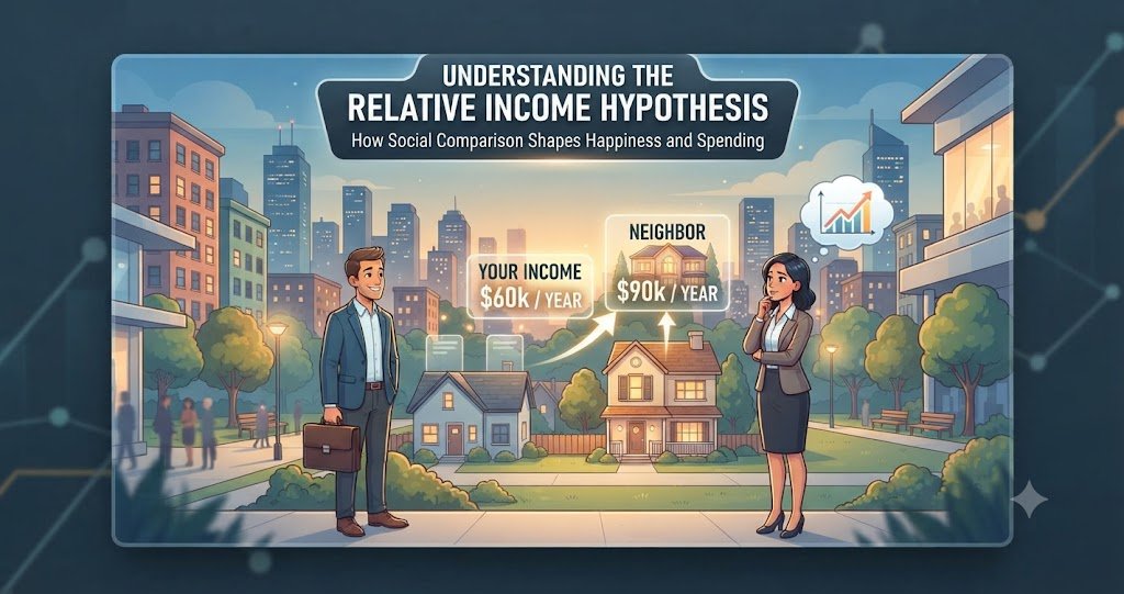
Relative Income Hypothesis
How Social Comparison Shapes Consumption
Why do two families earning the exact same income spend such different amounts on consumption? Why does a household that loses part of its income during a recession still find it so hard to cut back on spending? These questions puzzled economists for decades, and one of the most compelling answers came from American economist James Duesenberry through his Relative Income Hypothesis (RIH).
This article explains the background, assumptions, versions, mathematical formulation, and shortcomings of the Relative Income Hypothesis in simple academic language suitable for BS Economics students.
Background: The Consumption Puzzle
To understand why Duesenberry developed his theory, we first need to understand the problem he was trying to solve. According to John Maynard Keynes, absolute income is the primary determinant of consumption. As income rises, consumption moves upward along the same consumption function. Because of this, Keynes argued that the average propensity to consume (APC) falls as income rises. This can be written as:

However, economist Simon Kuznets empirically studied long-run consumption data in the United States and found something very different. He discovered that APC remained roughly constant at around 0.9 over the long run, regardless of how much income grew.
This contradiction between Keynes’ theoretical prediction (APC falls with income) and Kuznets’ empirical finding (APC stays constant) became known as the Consumption Puzzle. Several economists attempted to resolve this puzzle, and Duesenberry’s Relative Income Hypothesis was one of the earliest and most influential attempts.
Introduction to the Relative Income Hypothesis
James Duesenberry introduced this theory in 1949 in his book Income, Saving, and the Theory of Consumer Behavior. His central insight was simple but powerful: people do not evaluate their consumption in isolation. Instead, they compare themselves to others around them.
The Hypothesis: What Duesenberry Actually Argued
According to the Relative Income Hypothesis, the consumption of an individual is not a function of his absolute income. Instead, it depends on his income relative to the income of others in society.
This idea can be broken down into three key propositions:
- Absolute Income Rises: If the absolute income of all individuals rises by the same percentage, their relative positions in the income distribution remain unchanged.
- Relative Income Unchanged: Because relative positions stay the same, the fraction of income devoted to consumption does not change. APC stays constant.
- Consumption Function Shifts: As community income rises over time, the aggregate consumption function shifts upward rather than simply moving along a fixed function.
This is precisely how Duesenberry reconciled Keynes and Kuznets: in the short run, for a single household, higher relative income lowers APC (matching Keynes’ cross-section observation). But in the long run, as everyone’s income rises together, relative positions do not change, so APC remains constant (matching Kuznets’ time-series finding).
Numerical Example
Consider three families whose incomes all rise by 25%, keeping their relative positions in the income distribution unchanged.
| Family | Income Before | Consumption Before | APC Before | Income After (+25%) | Consumption After | APC After |
|---|---|---|---|---|---|---|
| Family A (Low) | Rs. 30,000 | Rs. 24,000 | 0.80 | Rs. 37,500 | Rs. 30,000 | 0.80 |
| Family B (Middle) | Rs. 60,000 | Rs. 48,000 | 0.80 | Rs. 75,000 | Rs. 60,000 | 0.80 |
| Family C (High) | Rs. 100,000 | Rs. 80,000 | 0.80 | Rs. 125,000 | Rs. 100,000 | 0.80 |
Each family began with an APC of 0.80 and ended with an APC of 0.80, even though their income rose substantially. Since relative positions in the income distribution remained unchanged, APC also remained unchanged.
Two Versions of the Relative Income Hypothesis
Duesenberry’s theory has two distinct versions: one that applies to cross-section data (comparing different households at the same point in time) and one that applies to time-series data (comparing the same household or economy over time). These correspond to two important effects: the Demonstration Effect and the Ratchet Effect.
The Demonstration Effect
The Demonstration Effect, also known as the Duesenberry Effect, explains cross-section behavior. It suggests that individuals and households try to imitate or copy the consumption expenditure patterns of their neighbors or reference group in order to maintain social status.
Two important implications follow from this effect:
APC Does Not Fall: If the incomes of all families increase in the same proportion, the distribution of relative incomes remains unchanged. Therefore, the proportion of income spent on consumption (APC) remains constant.
Relative Position Matters: A family devotes more of its income to consumption if it lives in a community where that income level is considered relatively low, because the demonstration effect is strong. Conversely, if the same income is considered relatively high within its community, the family spends a lower proportion of it, because the demonstration effect is weak or absent.
Example: A family earning Rs. 80,000 per month in an elite neighborhood, where the average income is Rs. 200,000, spends Rs. 74,000 (APC = 0.925) trying to keep up with wealthier neighbors. The same family, if it lived instead in a modest neighborhood where the average income is Rs. 50,000, would spend only Rs. 60,000 (APC = 0.75), since it already feels relatively well-off.
Explanation of the Demonstration Effect through a Diagram
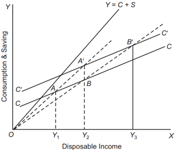
Suppose that Family A has Y1 level of income and consumption is Y1A. Suppose its income level rises to Y2. Now its consumption would not rise to Y2B but to Y2A’, where A’ lies on the same ray from the origin as the previous point A. It is because, according to Duesenberry, consumption increases in the same proportion as its income increases, with the result that APC remains constant.
Likewise, family B’s consumption will increase to Y3B’ when its income increases from Y2 to Y3, so that the APC of family B remains constant. If we join these A’ and B’ points, we will get a new consumption function C’ C’.
The Ratchet Effect
The Ratchet Effect explains time-series behavior, particularly what happens during economic downturns. It suggests that when the income of individuals or households falls, their consumption expenditure does not fall by a similar amount. In other words, the consumption function is irreversible, at least in the short run.
Two main reasons explain the Ratchet Effect:
Demonstration Effect (Social Pressure): People do not want their neighbors to know that their living standard has fallen. They continue spending at a similar level to maintain an image of prosperity.
Habit Formation: Once households reach a high standard of living, it becomes psychologically very difficult to cut back on consumption. They become accustomed to certain goods and services, such as premium brands and vacations, and are reluctant to give them up.
Example: A family accustomed to annual vacations and regular restaurant meals will save less, or rely on credit, during a salary cut rather than immediately cancel these habitual expenses.
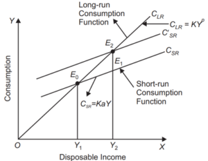
Explanation of the Ratchet Effect through a Diagram
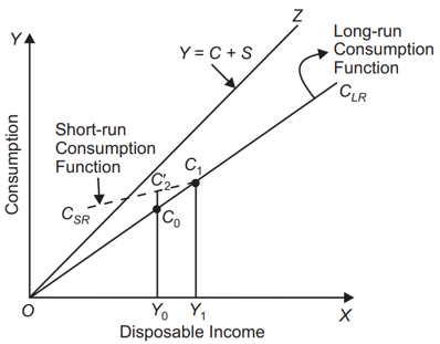
On the X-axis we measure disposable income and on the Y-axis the consumption and savings. Starting with disposable income of zero, we assume that there is steady growth of disposable income till it reaches Y1. The linear consumption function CLR is the long-run consumption function. It will be seen from the figure that at Y1 level of disposable income, the consumption expenditure equals Y1C1.
Now suppose with initial income level Y1, there is recession in the economy with the result that disposable income falls to the level Y0. According to Duesenberry, consumption would not fall greatly to the level Y0C0 as the long-run consumption function curve CLR would suggest. To maintain their consumption level previously reached people would now save less and reduce their consumption level only slightly to Y0C2` whereas point C2` is on the short-run consumption function curve CSR.
The Duesenberry Consumption Function
Duesenberry expressed his theory mathematically as:

| Symbol | Stands For | Explanation |
|---|---|---|
| APC = Cₜ/Yₜ | Average Propensity to Consume | Ratio of current consumption to current income |
| a | Autonomous constant | A positive constant greater than 1; represents the theoretical baseline APC when Yₜ/Y₀ equals zero |
| c | Marginal coefficient | A positive fraction between 0 and 1; as Yₜ/Y₀ rises, APC falls by c per unit |
| Yₜ | Current disposable income | The household’s actual income in the current period |
| Y₀ | Previous peak income | The highest income level the household has ever achieved; acts as a reference benchmark |
This equation shows that the ratio of current consumption to current income depends on the ratio of current income to the previous peak income. If this ratio stays constant, then the consumption-income ratio also stays constant. However, during a recession, when current income Yt falls below the previous peak income Y0, the current consumption-to-income ratio Ct/Yt rises, since households resist cutting consumption in line with falling income.
Shortcomings of the Relative Income Hypothesis
While influential, the Relative Income Hypothesis has several limitations that later economists pointed out:
- Reversibility of Consumption Patterns: RIH overemphasizes the irreversibility of consumption. In reality, if income remains low permanently, households do eventually adjust and cut consumption over the long term.
- Disproportionate Response to Income Increases: The theory inaccurately assumes a strictly proportional relationship between income increases and consumption increases.
- Non-Direct Relationship in Recessions: RIH fails to capture the full complexity of economic downturns. Factors such as government transfers, unemployment benefits, access to credit, and precautionary saving also shape household behavior, not just imitation and habit.
- Neglect of Broader Economic Factors: RIH ignores several important determinants of consumption, including age and life stage, urbanization, asset holdings, wealth effects, credit access, and household composition.
- Independent Consumer Preferences: Not all consumers blindly imitate their neighbors. Individual preferences, education, cultural values, and personal risk tolerance also shape consumption independently of peer behavior.
- Role of Income Expectations: RIH does not fully account for how expectations about future income shape current spending decisions. This gap was later addressed by Milton Friedman’s Permanent Income Hypothesis and Franco Modigliani’s Life-Cycle Hypothesis.
Example: A medical student living on a low stipend may borrow and spend heavily today, anticipating a high future income once training is complete. RIH, which focuses on relative social comparison rather than future expectations, cannot fully explain this behavior.
Comparison: Relative Income Hypothesis vs Absolute Income Hypothesis
| Feature | Absolute Income Hypothesis (Keynes) | Relative Income Hypothesis (Duesenberry) |
|---|---|---|
| Main determinant of consumption | Household’s own absolute income level | Household’s income relative to others in society |
| Behavior of APC | Falls as income rises | Remains constant as income rises proportionally |
| Consumption function | Fixed, with movement along the same curve | Shifts upward over time as community income rises |
| Reversibility | Consumption falls when income falls | Consumption is largely irreversible (ratchet effect) |
| Explains cross-section data | Weakly | Strongly (demonstration effect) |
| Explains time-series data | Weakly (contradicted by Kuznets) | Strongly (ratchet effect) |
| Role of social comparison | Not considered | Central to the theory |
Conclusion
The Relative Income Hypothesis marked a major step forward in consumption theory because it introduced the idea that social context, not just personal income, shapes how households spend and save. Through the demonstration effect, Duesenberry explained why households in different social settings behave differently even with identical incomes. Through the ratchet effect, he explained why consumption resists falling during recessions. Together, these insights successfully resolved the Consumption Puzzle between Keynes and Kuznets. Although later theories such as the Permanent Income Hypothesis and Life-Cycle Hypothesis addressed some of its limitations, particularly around income expectations, the Relative Income Hypothesis remains a foundational concept in the study of consumer behavior and macroeconomics.
Suggestions for Further Readings:


 MinhajMetricsHub
2 responses to “Relative Income Hypothesis: Duesenberry’s Theory of Consumption Explained”
[…] Relative Income Hypothesis: Duesenberry’s Theory of Consumption Explained […]
[…] Duesenberry in his Relative Income Hypothesis, said that spending depends on how a person’s income compares to other people’s income […]