Box-Jenkins Methodology: Complete ARIMA Forecasting Guide

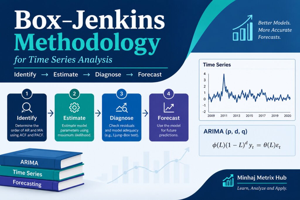
Forecasting is one of the oldest and most practical tasks in applied economics. Whether we are projecting inflation, exchange rates, GDP growth, or electricity demand, we need a disciplined way to move from raw data to a defensible forecast.

The Box-Jenkins methodology is exactly such a framework. First set out by George E. P. Box and Gwilym M. Jenkins in their book Time Series Analysis: Forecasting and Control (1970), it remains the standard recipe for building ARIMA models more than five decades later.

This article is a complete, step-by-step guide to the methodology. We begin with the building blocks of an ARIMA(p, d, q) model, walk through the four stages of the approach (identification, estimation, diagnostic checking and forecasting) using a worked Consumer Price Index (CPI) example, and finish with a brief introduction to the most useful variants of the ARIMA family.

Table of Contents

What is the Box-Jenkins methodology?

The Box-Jenkins methodology is an iterative, data-driven procedure for finding the ARIMA model that best describes a univariate time series and then using that model to forecast. Unlike structural econometric models, which rely on economic theory to select explanatory variables, a Box-Jenkins model lets the series “speak for itself”: the future values of a variable are explained only by its own past values and by past random shocks.

Two features make the approach attractive. First, it is parsimonious: a handful of parameters can capture rich dynamics. Second, it is self-checking: the methodology includes a formal diagnostic stage, and if the model fails, we return to the first stage and try again. This identify, estimate, check, and revise loop is the core of the approach.

The ARIMA(p, d, q) model

An ARIMA model combines three components, each governed by one integer parameter:

AR (p), Autoregressive: the current value depends linearly on its own $p$ previous values.
I (d), Integrated: the series must be differenced $d$ times to become stationary.
MA (q), Moving Average: the current value depends on the current and $q$ previous random shocks (error terms).

Stationarity: the prerequisite

A time series $Y_t$ is (weakly) stationary if its mean and variance are constant over time and its autocovariance depends only on the lag between observations and not on time itself. Economic series such as prices, GDP and money supply typically trend upward and are therefore non-stationary in levels. A series that becomes stationary after differencing $d$ times is said to be integrated of order d, written $I(d)$ .

The first difference of a series is

$\Delta Y_t = Y_t - Y_{t-1}$

and the $d$ -th difference is obtained by applying the operator $d$ times. If the series is stationary at level, $d = 0$ ; if it becomes stationary after first differencing, $d = 1$ , and so on. In practice $d$ is rarely larger than 2.

General form of the ARIMA(p, d, q) model

Let $w_t = \Delta^{d} Y_t$ denote the series after differencing $d$ times. The ARIMA(p, d, q) model for $Y_t$ is an ARMA(p, q) model for $w_t$ :

$w_t = \gamma_0 + \sum_{i=1}^{p}\alpha_i w_{t-i} + \sum_{i=1}^{q}\beta_i \varepsilon_{t-i} + \varepsilon_t$

where $\gamma_0$ is a constant, $\alpha_i$ are the autoregressive coefficients, $\beta_i$ are the moving-average coefficients and $\varepsilon_t$ is a white-noise error term with zero mean and constant variance $\sigma^2$ . When $d = 0$ , $w_t = Y_t$ and the expression reduces to the familiar ARMA(p, q) model.

The same model can be written compactly with the backshift (lag) operator $B$ , defined by $BY_t = Y_{t-1}$ :

$\alpha(B)(1-B)^{d}Y_t = \gamma_0 + \beta(B)\varepsilon_t$

where $\alpha(B) = 1 - \alpha_1 B - \alpha_2 B^2 - \cdots - \alpha_p B^p$ and $\beta(B) = 1 + \beta_1 B + \beta_2 B^2 + \cdots + \beta_q B^q$ .

Two special cases: an ARIMA(p, d, 0) model is a pure autoregressive model of the differenced series, and an ARIMA(0, d, q) model is a pure moving-average model of the differenced series. An ARIMA(0, 1, 0) model is the random walk (with drift if a constant is included).

Note on conventions: software packages parameterise the constant differently. For example, in EViews the reported constant C in an ARMA model is the mean of the differenced series, not the intercept $\gamma_0$ in the equation above. Always check the documentation of your software before interpreting the constant.

The four steps at a glance

Table 1: 4 Steps of Box-Jenkins Methodology

Step	Purpose	Main tools
1. Identification	Decide the orders $p$ , $d$ and $q$	Line plot, correlogram (ACF and PACF), unit root tests (ADF, PP, KPSS)
2. Estimation	Estimate the parameters of the candidate models and select the best one	OLS, maximum likelihood; AIC, SBC, HQC; significance of coefficients
3. Diagnostic checking	Verify that the residuals are white noise and that the model is stable	Residual correlogram, Ljung-Box Q test, inverse AR/MA roots
4. Forecasting	Predict future values and evaluate accuracy	MAE, MSE, RMSE, MAPE

If the model fails the diagnostic stage, we return to Step 1 or Step 2, revise the specification and repeat the cycle.

Step 1: Identification

The aim of this step is to determine the appropriate values of $d$ , $p$ and $q$ . We start with $d$ because the ACF and PACF can only be interpreted properly for a stationary series.

1A. Check for stationarity (determine d)

Three complementary tools are used.

(i) Line plot. Plot the series against time. An upward or downward trend, a changing variance or regular periodic swings are warning signs of non-stationarity.

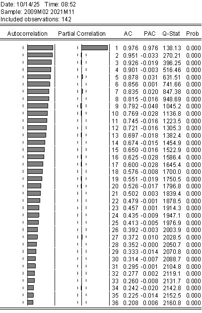
(ii) Correlogram. The autocorrelation function (ACF) and partial autocorrelation function (PACF) of a non-stationary series have a characteristic look: the ACF decays very slowly and stays significant across many lags, while the PACF shows a single dominant spike at lag 1 (close to one) and then cuts off.

(iii) Unit root tests. The formal test is the Augmented Dickey-Fuller (ADF) test (or the Phillips-Perron, PP, test). The ADF regression is

$\Delta Y_t = a_0 + a_1 t + \gamma Y_{t-1} + \sum_{i=1}^{k}\delta_i \Delta Y_{t-i} + u_t$

where $a_0$ is a constant, $a_1 t$ is a deterministic trend (included when the series visibly trends) and the lagged differences $\Delta Y_{t-i}$ absorb serial correlation in the errors. The hypotheses are:

$H_0: \gamma = 0 \ \text{(the series has a unit root, i.e. is non-stationary)} \qquad H_1: \gamma \text{ is negative (the series is stationary)}$

Reject $H_0$ if the p-value is less than 0.05 (equivalently, if the test statistic is more negative than the critical value) and conclude that the series is stationary. Otherwise, do not reject $H_0$ , difference the series and test again. Because the ADF and PP tests have low power against near-unit-root alternatives, it is good practice to confirm the result with the KPSS test, whose null hypothesis is stationarity.

Worked example: Consumer Price Index (CPI)

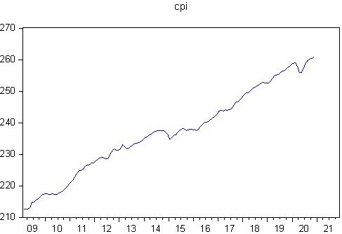
We use monthly CPI data from 2009M03 to 2020M11. Three pieces of evidence are examined:

Line plot: CPI rises steadily over the sample, a clear trend that suggests non-stationarity.

Correlogram: the ACF of the level series decays slowly and the PACF cuts off after lag 1, as described above.

ADF test (constant and linear trend, lag length chosen by SIC): the test statistic is -2.3231 with a p-value of 0.4184, against a 5% critical value of -3.4425. We cannot reject the null hypothesis, so CPI has a unit root.

Null Hypothesis: CPI has a unit root

Exogenous: Constant, Linear Trend

Lag Length: 2 (Automatic – based on SIC, maxlag=13)

	t-Statistic	Prob.*
Augmented Dickey-Fuller test statistic	-2.323145	0.4184
Test critical values:
1% level	-4.025426
5% level	-3.442474
10% level	-3.145882

We therefore difference the series once. The ADF test on D(CPI) gives a statistic of -7.7642 with p-value 0.0000, which is far below the 1% critical value of -4.0254. The null of a unit root is rejected, so the differenced series is stationary and CPI is integrated of order one, $I(1)$ . Hence $d = 1$ .

Null Hypothesis: D(CPI) has a unit root

Exogenous: Constant, Linear Trend

Lag Length: 1 (Automatic – based on SIC, maxlag=13)

	t-Statistic	Prob.*
Augmented Dickey-Fuller test statistic	-7.764199	0.0000
Test critical values:
1% level	-4.025426
5% level	-3.442474
10% level	-3.145882

Technical note: the trend term is appropriate for CPI in levels, but a differenced series no longer trends, so a constant-only ADF specification is normally used for D(CPI). With a statistic as extreme as -7.76, the conclusion is not affected.

A caution on over-differencing. Differencing more than necessary introduces artificial negative autocorrelation (a spike near -0.5 at lag 1 of the ACF) and inflates the forecast variance. Difference only until stationarity is achieved. If the series shows a seasonal pattern, seasonal differencing may also be required (see SARIMA below). If the variance grows with the level of the series, a log transformation before differencing is usually appropriate.

1B. Identify the p and q terms

Once the series is stationary, examine the correlogram of the differenced series. The theoretical patterns of the ACF and PACF for the basic processes are summarised below.

Process	ACF	PACF
AR(p)	Tails off (geometric or damped sinusoidal decay)	Cuts off after lag $p$
MA(q)	Cuts off after lag $q$	Tails off
ARMA(p, q)	Tails off after lag $q$	Tails off after lag $p$

Rule of thumb: use the PACF to suggest the AR order $p$ and the ACF to suggest the MA order $q$ . A spike is regarded as significant when it lies outside the approximate confidence bands of $\pm 1.96/\sqrt{T}$ , where $T$ is the number of observations.

In practice the sample ACF and PACF are noisy and rarely match a textbook pattern exactly. They often suggest several plausible models. The Box-Jenkins advice is to consider all reasonable candidates and estimate each of them, rather than agonising over a single “correct” choice.

Worked example (continued)

With $T = 141$ observations, the approximate 95% band is $\pm 1.96/\sqrt{141} \approx \pm 0.165$ . The correlogram of D(CPI) shows a large first autocorrelation (0.391) and a significant negative autocorrelation at lag 3 (-0.202), with the rest mostly inside the band; the partial autocorrelations are 0.391 and -0.186 at lags 1 and 2, and -0.156 at lag 3 (borderline). The Q-statistics are significant at every lag, confirming that D(CPI) is autocorrelated and worth modelling.

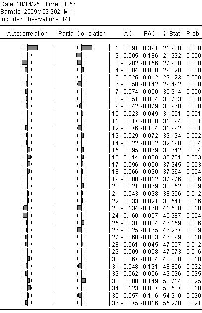
The pattern does not match a single textbook process, so it points to a short AR term together with an MA term at lag 3. We retain two candidates:

ARIMA(1, 1, 1)
ARIMA(1, 1, 3)

Step 2: Estimation

Each candidate model is now estimated. Because ARMA models contain lagged error terms, which are unobserved, ordinary least squares is generally not appropriate for models with MA terms. The usual methods are:

Maximum likelihood estimation (MLE), the most widely used method, which assumes normally distributed errors and maximises the likelihood function numerically;
Conditional least squares, which sets the pre-sample errors to zero and minimises the sum of squared residuals;
OLS, which is valid for pure AR models.

Numerical estimation can fail to converge or may converge to a poor solution, so check the convergence message in your output.

Choosing the best model

After estimating the candidate models, we choose the one that fits the data well using the following criteria:

Minimum information criteria: the Akaike (AIC), Schwarz/Bayesian (SBC or BIC) and Hannan-Quinn (HQC) criteria. They reward goodness of fit and penalise additional parameters.
Maximum adjusted $R^2$ .
Statistical significance of the estimated coefficients (number of significant coefficients).
Parsimony: among models that fit similarly, prefer the one with fewer parameters.

In the per-observation form reported by packages such as EViews, the criteria are

$AIC = \frac{-2\ln L + 2k}{T}, \qquad SBC = \frac{-2\ln L + k\ln T}{T}, \qquad HQC = \frac{-2\ln L + 2k\ln(\ln T)}{T}$

where $L$ is the maximised likelihood, $k$ the number of estimated parameters and $T$ the number of observations. Smaller values indicate a better trade-off between fit and complexity. SBC penalises extra parameters most heavily and therefore tends to select smaller models than AIC.

Note that information criteria are comparable only across models estimated on the same sample and the same dependent variable, which also means the same order of differencing $d$ . You cannot use AIC to choose between an ARIMA(1, 1, 1) and an ARIMA(1, 0, 1) model, because their dependent variables ( $\Delta Y_t$ versus $Y_t$ ) differ. Likewise, adjusted $R^2$ and the count of significant coefficients are only informal guides in ARMA models; the information criteria and the diagnostic tests in Step 3 carry more weight.

Worked example (continued)

Both models are estimated by maximum likelihood on D(CPI) with 141 observations.

Variable	ARIMA(1, 1, 1): coefficient (p-value)	ARIMA(1, 1, 3): coefficient (p-value)
C	0.3399 (0.0000)	0.3411 (0.0000)
AR(1)	0.2023 (0.2545)	0.4129 (0.0000)
MA(1)	0.2398 (0.1930)	not included
MA(3)	not included	-0.2990 (0.0011)
SIGMASQ	0.2207 (0.0000)	0.2095 (0.0000)

In the ARIMA(1, 1, 3) specification, the AR(1) and MA(3) terms are included and the insignificant MA(1) and MA(2) terms are omitted (a “subset” or “restricted” ARIMA model). Note that in ARIMA(1, 1, 1) neither the AR(1) nor the MA(1) coefficient is statistically significant.

Criterion	ARIMA(1, 1, 1)	ARIMA(1, 1, 3)	Preferred
Akaike (AIC)	1.3848	1.3345	ARIMA(1, 1, 3)
Schwarz (SBC)	1.4685	1.4181	ARIMA(1, 1, 3)
Hannan-Quinn (HQC)	1.4188	1.3684	ARIMA(1, 1, 3)
Adjusted $R^2$	0.1516	0.1946	ARIMA(1, 1, 3)
Significant coefficients	Only the constant	All coefficients	ARIMA(1, 1, 3)

ARIMA(1, 1, 3) wins on every criterion, so it is our preferred model. Before we use it, it must pass the diagnostic checks.

Step 3: Diagnostic checking

A good ARIMA model should extract all the systematic information from the data and leave behind only unpredictable noise. Diagnostic checking therefore asks: are the residuals white noise?

3A. Residual correlogram and the Ljung-Box Q test

Plot the ACF and PACF of the residuals. If the model is adequate, all autocorrelations should lie within the confidence bands. The formal test is the Ljung-Box Q test, with hypotheses

$H_0: \text{Residuals are white noise (no autocorrelation up to lag } h) \qquad H_1: \text{Residuals are not white noise}$

and test statistic

$Q = T(T+2)\sum_{k=1}^{h}\frac{\hat{\rho}_k^{2}}{T-k}$

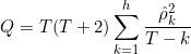
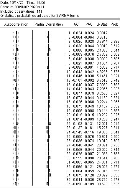
where $\hat{\rho}_k$ is the residual autocorrelation at lag $k$ . Under $H_0$ , $Q$ follows approximately a chi-square distribution with $h - p - q$ degrees of freedom. If the p-values of the Q-statistics are greater than 0.05 at all (or, allowing for the occasional chance rejection at long lags, essentially all) lags, we do not reject $H_0$ , and the residuals are not autocorrelated. Otherwise, the model has missed some dynamics and needs to be revised, for instance by adding AR or MA terms.

Example: for the ARIMA(1, 1, 3) model, the Q-statistic p-values at lags 3 to 36 all lie between 0.38 and 0.95, well above 0.05. The residuals show no remaining serial correlation, so the model passes the test.

3B. Stability: AR and MA roots

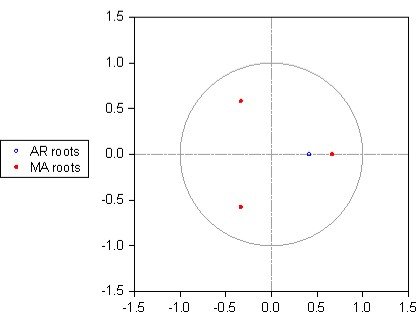
The estimated model must be stable. Stationarity requires that all roots of $\alpha(B) = 0$ lie outside the unit circle, which is the same as saying that the inverse AR roots (the ones reported by software such as EViews) lie inside the unit circle.

Invertibility of the MA part requires the same for the inverse MA roots. Packages usually display these as a graph of the inverse roots against the unit circle. In our example, the inverse AR root is 0.41, and the inverse MA roots are 0.67 and -0.33 ± 0.58i, all of modulus less than one, so the model is stable and invertible.

3C. Additional checks

Normality of residuals (Jarque-Bera test), which matters mainly for the validity of forecast intervals.
Heteroskedasticity (ARCH-LM test on residuals). Significant ARCH effects, common in financial series, suggest combining ARIMA with a GARCH model.
Overfitting: add an extra AR or MA term. If it is insignificant and the criteria do not improve, the original model is adequate.

If the model passes the diagnostic tests, we proceed to forecasting. If several models pass, we can compare their forecasting performance.

Step 4: Forecasting

The ultimate purpose of most ARIMA modelling is forecasting. Given the data up to time $T$ , the $h$ -step-ahead forecast is the conditional expectation

$\hat{Y}_{T+h} = E\left[Y_{T+h} \mid Y_T, Y_{T-1}, \ldots\right]$

It is computed recursively: future errors are replaced by their expected value (zero), past errors by the model residuals, and future values of the series by their own forecasts. For an integrated series, the forecasts of the differences are accumulated back to the level of the series. With $d = 1$ , for example,

$\hat{Y}_{T+h} = Y_T + \hat{w}_{T+1} + \hat{w}_{T+2} + \cdots + \hat{w}_{T+h}$

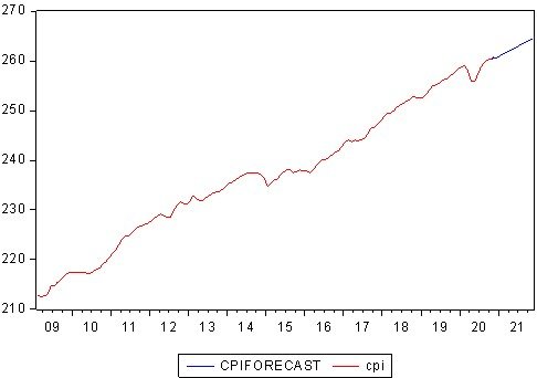
Two features of ARIMA forecasts are worth remembering. First, as the horizon grows, the forecast of a stationary differenced series converges to its mean, so for a model with $d = 1$ and a non-zero mean, the long-run forecast is a straight line with slope equal to that mean. This is exactly the shape of the CPI forecast in our example. Second, the forecast error variance increases with the horizon, so prediction intervals fan out. A $(1-\alpha)$ interval takes the form

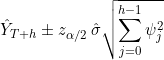
$\hat{Y}_{T+h} \pm z_{\alpha/2}\,\hat{\sigma}\sqrt{\sum_{j=0}^{h-1}\psi_j^{2}}$

where $\psi_j$ are the coefficients of the infinite moving-average representation of the integrated process.

Measuring forecast accuracy

Let $e_t = Y_t - \hat{Y}_t$ be the forecast error over $n$ forecast periods. The commonly used accuracy measures are:

$MAE = \frac{1}{n}\sum_{t=1}^{n}\left|e_t\right| \qquad MSE = \frac{1}{n}\sum_{t=1}^{n}e_t^{2} \qquad RMSE = \sqrt{MSE} \qquad MAPE = \frac{100}{n}\sum_{t=1}^{n}\left|\frac{e_t}{Y_t}\right|$

MAE is the average absolute error, in the units of the data.
MSE and RMSE penalise large errors more heavily; RMSE is in the units of the data.
MAPE is scale-free (percentage) and therefore convenient for comparing across series, but it is undefined when the series takes the value zero.

The model that minimises these statistics has the best forecasting accuracy. For a fair assessment, evaluate forecasts on a hold-out sample that was not used in estimation (out-of-sample evaluation), since in-sample fit can be flattering.

Worked example (continued)

Measure	ARIMA(1, 1, 3)	ARIMA(1, 1, 1)
RMSE	2.1764	2.3104
MAE	1.8210	1.9274
MAPE (%)	0.7755	0.8206

ARIMA(1, 1, 3) has the smaller RMSE, MAE and MAPE, so it is also the more accurate of the two models on this evaluation. Three cautions apply when reading these numbers:

The gap is small. Whether a difference in RMSE is statistically meaningful should be tested formally, for example with the Diebold-Mariano test.
Check what kind of forecast was evaluated. The forecast sample (2009M02 to 2021M11) overlaps almost entirely with the estimation sample (to 2020M11), and the forecast line is a straight line from 2009 onwards, which is what a dynamic multi-step forecast of an ARIMA(p, 1, q) model with drift looks like. Such statistics describe how well the model’s long-run trend tracks the data, not genuine one-step-ahead or out-of-sample accuracy. For a proper assessment, re-estimate on a shorter sample and compare forecasts with the held-out observations (for example the last 12 months).
Benchmark against a naive forecast. The Theil U2 coefficients reported in the output (about 3.6 and 3.8) are above one, which signals that a simple no-change forecast would do better over that evaluation. A good forecast evaluation always compares the model with a simple benchmark.

With these caveats, the MAPE of about 0.78% says that the fitted path deviates from actual CPI by under one percent on average, which is encouraging but not a guarantee of future accuracy.

Common pitfalls

Skipping the stationarity check. Fitting ARMA terms to a trending series produces spurious results.
Over-differencing. It adds noise and artificial MA structure.
Relying on the correlogram alone. Use it to generate candidates, then let information criteria and diagnostics decide.
Over-parameterisation. Models with many insignificant terms fit the sample but forecast poorly, and cancelling AR and MA roots signal redundancy.
Ignoring structural breaks. Breaks (policy changes, crises, COVID-19) can mimic unit roots and distort identification.
Treating long-horizon forecasts as precise. Always report prediction intervals.

Variants of the ARIMA model useful for forecasting

The basic ARIMA model has been extended in many directions to handle seasonality, external information, long memory and time-varying volatility. The Box-Jenkins cycle of identification, estimation, diagnostics and forecasting carries over to all of them.

1. AR, MA and ARMA models

These are the special cases of ARIMA for stationary series ( $d = 0$ ). AR(p) models suit series with persistence, MA(q) models suit series with short-lived shocks, and ARMA(p, q) combines both with fewer parameters than a pure AR or MA model would need.

2. ARIMA with drift

Including a constant in an ARIMA model with $d = 1$ adds a deterministic drift to the stochastic trend. It is appropriate for series such as GDP or price indices that grow at a roughly constant average rate, and is the reason the CPI forecast above slopes upward.

3. SARIMA (Seasonal ARIMA)

Monthly or quarterly data often repeat a pattern every $s$ periods ( $s = 12$ for monthly data, $s = 4$ for quarterly data). The seasonal ARIMA model, written ARIMA(p, d, q)(P, D, Q) $_s$ , adds seasonal AR, differencing and MA terms:

$\Phi(B^{s})\,\alpha(B)\,(1-B)^{d}(1-B^{s})^{D}\,Y_t = \gamma_0 + \Theta(B^{s})\,\beta(B)\,\varepsilon_t$

It is the natural choice for retail sales, tourist arrivals, electricity demand or agricultural prices, where seasonality is strong.

4. ARIMAX and SARIMAX

These models add exogenous regressors $X_t$ (for example interest rates, policy dummies or weather variables) to the ARIMA structure:

$w_t = \gamma_0 + \delta' X_t + \sum_{i=1}^{p}\alpha_i w_{t-i} + \sum_{i=1}^{q}\beta_i \varepsilon_{t-i} + \varepsilon_t$

They are useful when relevant explanatory information is available, with two caveats: future values of $X_t$ must be known or forecast as well, and the regressors should be stationary (or differenced in the same way as $Y_t$ ) so that the equation does not mix integrated and stationary variables. Intervention analysis and dummy variables for outliers and structural breaks fall under this heading.

5. ARFIMA (Fractionally Integrated ARMA)

Standard ARIMA models allow only integer orders of differencing. ARFIMA(p, d, q) allows $d$ to be a fraction, which captures long memory, i.e. autocorrelations that decay slowly (hyperbolically) rather than exponentially. It is used for inflation, volatility and some hydrological and financial series.

6. ARIMA-GARCH

ARIMA models assume a constant error variance. When the residuals show volatility clustering (large shocks followed by large shocks), as in stock returns and exchange rates, the ARIMA model for the conditional mean is combined with a GARCH model for the conditional variance. The point forecasts come from the ARIMA part, while the GARCH part produces more realistic, time-varying forecast intervals.

7. Multivariate extensions: VAR, VARMA and VECM

When several series interact, the univariate approach is extended to vectors. Vector autoregressions (VAR) and vector ARMA (VARMA) models forecast several variables jointly, and the vector error-correction model (VECM) is used when the variables are cointegrated.

8. Automated ARIMA (auto-ARIMA)

Algorithms such as auto.arima() in R and pmdarima in Python automate the identification and estimation steps by searching over many (p, d, q) combinations and choosing the one with the lowest AICc. They are a convenient benchmark and a time saver for large numbers of series, but they do not replace diagnostic checking or economic judgement.

Model	Extension	Typical use
ARMA	Stationary series, $d = 0$	Interest-rate spreads, growth rates
ARIMA with drift	Constant added after differencing	GDP, price indices
SARIMA	Seasonal AR, MA and differencing	Monthly sales, electricity demand
ARIMAX / SARIMAX	External regressors	Forecasts with policy or weather variables
ARFIMA	Fractional differencing	Long-memory series
ARIMA-GARCH	Time-varying variance	Financial returns, exchange rates
VAR / VARMA / VECM	Several interacting series	Macroeconomic systems

Conclusion

The Box-Jenkins methodology gives us a systematic, transparent route from raw data to forecasts. In summary:

Identify: make the series stationary (choose $d$ using plots, correlograms and ADF/PP tests), then read the ACF and PACF to propose candidate values of $p$ and $q$ .
Estimate: fit all candidate models by maximum likelihood and select the best using AIC, SBC, HQC, adjusted $R^2$ , significance and parsimony.
Diagnose: confirm that the residuals are white noise (Ljung-Box test) and that the inverse AR and MA roots lie inside the unit circle. If not, revise the model.
Forecast: generate forecasts with prediction intervals and judge accuracy with MAE, RMSE and MAPE.

In our CPI example, the series was integrated of order one, the correlogram suggested two candidate models, and ARIMA(1, 1, 3) was preferred on all selection criteria, passed all residual diagnostics and delivered the lower forecast errors. Whenever seasonality, exogenous drivers, long memory or volatility clustering are present, the extensions discussed above allow the same workflow to be applied to richer problems.

If you found this guide useful, share it with your classmates and leave a comment below with the topics you would like me to cover next, such as the ADF test in detail, SARIMA modelling or ARCH/GARCH models.

References

Box, G. E. P., Jenkins, G. M., Reinsel, G. C., & Ljung, G. M. (2015). Time Series Analysis: Forecasting and Control (5th ed.). Hoboken, NJ: Wiley.
Dickey, D. A., & Fuller, W. A. (1979). Distribution of the estimators for autoregressive time series with a unit root. Journal of the American Statistical Association, 74(366), 427-431.
Enders, W. (2014). Applied Econometric Time Series (4th ed.). Hoboken, NJ: Wiley.

Share this article

About the author

Muhammad Minhaj Akhtar

Muhammad Minhaj Akhtar is a Lecturer in Economics at Government Graduate College Jauharabad, Pakistan. He holds an M.Phil. in Economics from Quaid-i-Azam University, Islamabad, and an MSc in Economics from the University of Sargodha, where he earned a Silver Medal. His academic passion lies in Econometrics, with a strong focus on applying empirical methods to real-world economic issues. Through MinhajMetrixHub, he shares learning resources, research guidance, and practical econometric insights for students and researchers.