

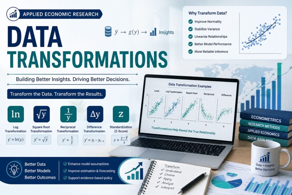
Data transformations are one of the most important steps in applied economics. Before any economic variable, say GDP, inflation, wages, or trade, can be used in a model, it usually needs to be changed in some way. Raw data is rarely ready to use as it comes. This article explains the main data transformations used by economists and researchers, why each one is needed, and how it is applied in practice.
Why Data Transformations Matter
Every applied economic question, from the effect of a tax policy to the return on education, is answered by fitting a model to data. But raw variables often have problems: they may grow over time (trend), swing with the seasons, be measured in different units, or contain extreme outliers. If these problems are not fixed first, the results of a model can be misleading or even meaningless. This is why choosing the right data transformation is a key step, not an optional one, in any economic analysis.
1. Index Numbers
An index number shows the relative change in a value, such as price or quantity, from one time period to another, compared to a chosen base period. Familiar examples are the Consumer Price Index (CPI) and the Producer Price Index (PPI).
By convention, the base period is always set to 100. Every other period is expressed relative to it. For example, an index value of 112 means the variable has risen by 12% since the base period.
Two index series can only be compared directly if they share the same base year. When two index series use different base years, they must first be converted to a common base year. This process is called splicing.
Worked Example of Splicing
| Year | Index (1985 = 100) | Index (1990 = 100) | Spliced (1990 = 100) |
|---|---|---|---|
| 1985 | 100.0 | — | 45.9 |
| 1987 | 142.0 | — | 65.1 |
| 1990 | 218.0 | 100.0 | 100.0 |
| 1991 | — | 108.0 | 108.0 |
| 1992 | — | 119.0 | 119.0 |
The general rule is simple: multiply or divide the whole series by the factor needed to make the new base period equal to 100. In the example above, the 1985-based series is divided by  (the 1990 index value divided by 100) to rebase it to 1990.
2. Changing the Frequency of Time Series Data
Economic data is often collected at different time intervals such as weekly, monthly, quarterly, or annually. Changing between these frequencies is a common first step before modelling.
- Aggregating to a lower frequency (for example, weekly sales combined into monthly sales) smooths out noise and short-run randomness.
- Disaggregating to a higher frequency (for example, converting annual data into quarterly data) needs interpolation and is used when detailed data is not directly available.
The right frequency depends on the question being studied. Policy analysis often uses quarterly or annual data, while market analysis may need daily or even intraday data.
3. Nominal vs Real Data
Nominal data includes the effect of price changes (inflation), while real data removes this effect to show the true change in quantity or purchasing power. Comparing two nominal variables can create a false or “spurious” relationship, simply because both are being pushed up by inflation.
The formula to convert nominal data into real data is:
![\[\text{Real Value} = \left( \frac{\text{Nominal Value}}{\text{Price Deflator}} \right) \times 100\]](https://minhajmetrixhub.com/wp-content/ql-cache/quicklatex.com-e385febbc50896e1fc4e47f1209012eb_l3.png "Rendered by QuickLaTeX.com")
The deflator chosen should match the variable: the CPI for consumer spending, the PPI or WPI for production values, and the GDP deflator for national output. As a simple rule, if a variable is measured in currency and observed over more than a couple of years, it should usually be converted to real terms before being used in a regression alongside another currency-based variable. Common examples include wages, GDP, tax revenue, and consumption.
4. Logarithms: Why and When to Use Them
The natural logarithm (written as  ) is one of the most widely used transformations in economics. It is used for several reasons:
- It turns multiplicative and exponential relationships into straight-line (linear) relationships, so standard regression tools can be used.
- It stabilises variance and reduces heteroscedasticity in variables that grow proportionally, such as GDP, prices, population, and wages.
- It compresses the scale of the data, reducing the effect of extreme values and skewness.
- It gives coefficients a direct, easy-to-understand meaning as elasticities or percentage effects.
One important caution:  is undefined when
  . Variables that can be negative, such as profit or trade balance, cannot be logged directly. A common workaround for data that can be zero, such as counts, is to use
  , though this slightly changes the interpretation and should always be reported clearly.
Common Log-Based Model Forms
| Model | Specification | What the Coefficient ( ) Means ) Means |
|---|---|---|
| Log-Log |  | A 1% rise in  leads to a leads to a  change in change in  (constant elasticity) (constant elasticity) |
| Log-Lin (Semi-log) |  | A 1-unit rise in leads to a  change in change in |
| Lin-Log |  | A 1% rise in leads to a  unit change in unit change in |
| Linear (no log) |  | A 1-unit rise in leads to a -unit change in |
A classic example is the Mincer wage equation:  . Here, the coefficient on education is read directly as the approxmate percentage return to one extra year of schooling. This is why log-lin wage models are standard in labor economics.
5. Differencing
Differencing is used to remove a trend from a time series and to achieve stationarity — meaning the series has a constant mean and variance over time. This is essential because most raw economic time series are non-stationary, and using non-stationary data directly in a regression can lead to spurious results.
- First difference:
 — converts a level series into period-to-period change.
 - Second difference:
 — used when a series is integrated of order 2, meaning one difference is not enough to remove the trend.
 - Seasonal differencing:
 , where
  for quarterly data or
  for monthly data — removes a repeating seasonal pattern.
 — converts a level series into period-to-period change.
 — used when a series is integrated of order 2, meaning one difference is not enough to remove the trend.
 , where
  for quarterly data or
  for monthly data — removes a repeating seasonal pattern.
Before deciding whether a series needs differencing, researchers typically run the Augmented Dickey-Fuller (ADF) test to check for a unit root.
6. Growth Rates
Growth rates express change in comparable percentage terms, which is useful because different variables are often measured in different units.
- Simple growth rate:

- Log-difference approximation:
![g_t \approx [\ln(Y_t) - \ln(Y_{t-1})] \times 100](data:image/svg+xml;base64,PHN2ZyB4bWxucz0iaHR0cDovL3d3dy53My5vcmcvMjAwMC9zdmciIHdpZHRoPSIyMTAiIGhlaWdodD0iMTciIHZpZXdCb3g9IjAgMCAyMTAgMTciPjxyZWN0IHdpZHRoPSIxMDAlIiBoZWlnaHQ9IjEwMCUiIHN0eWxlPSJmaWxsOiNjZmQ0ZGI7ZmlsbC1vcGFjaXR5OiAwLjE7Ii8+PC9zdmc+ "Rendered by QuickLaTeX.com") , which is accurate for small changes and can be added across periods.
, which is accurate for small changes and can be added across periods. - Compound Annual Growth Rate (CAGR):
![\left[ \left( \dfrac{Y_t}{Y_0} \right)^{1/n} - 1 \right] \times 100](data:image/svg+xml;base64,PHN2ZyB4bWxucz0iaHR0cDovL3d3dy53My5vcmcvMjAwMC9zdmciIHdpZHRoPSIxNTUiIGhlaWdodD0iNTEiIHZpZXdCb3g9IjAgMCAxNTUgNTEiPjxyZWN0IHdpZHRoPSIxMDAlIiBoZWlnaHQ9IjEwMCUiIHN0eWxlPSJmaWxsOiNjZmQ0ZGI7ZmlsbC1vcGFjaXR5OiAwLjE7Ii8+PC9zdmc+ "Rendered by QuickLaTeX.com")
- Year-over-Year (YoY) growth: compares a period to the same period one year earlier, which automatically removes seasonality.
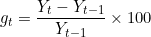
![g_t \approx [\ln(Y_t) - \ln(Y_{t-1})] \times 100](https://minhajmetrixhub.com/wp-content/ql-cache/quicklatex.com-beed5d7c57bbe7e0e71e44321a77b2a9_l3.png "Rendered by QuickLaTeX.com") , which is accurate for small changes and can be added across periods.
, which is accurate for small changes and can be added across periods.![\left[ \left( \dfrac{Y_t}{Y_0} \right)^{1/n} - 1 \right] \times 100](https://minhajmetrixhub.com/wp-content/ql-cache/quicklatex.com-6bd62bb491fd4aa4f70f0365594cb088_l3.png "Rendered by QuickLaTeX.com")
Growth rates allow GDP growth, inflation (CPI growth), and population growth to all be compared on the same footing, even though they start from very different units and scales.
7. Standardization and Centering
Standardisation (Z-scores) rescales a variable to have a mean of 0 and a standard deviation of 1, using the formula:
![\[Z_i = \frac{X_i - \text{mean}(X)}{\text{standard deviation}(X)}\]](https://minhajmetrixhub.com/wp-content/ql-cache/quicklatex.com-c917da903114ff1670c29acf10b3488b_l3.png "Rendered by QuickLaTeX.com")
This is useful when comparing variables measured in very different units, such as income, years of schooling, and test scores, and is commonly used when building composite indices, such as the Human Development Index (HDI).
Centring (demeaning) uses the formula  , which shifts the variable’s origin to zero without changing its spread. Centering reduces artificial multicollinearity between a variable and its interaction or quadratic term, and it is the basis of the panel-data “within” transformation used in fixed-effects estimation, where each unit’s own mean is subtracted to remove unit-specific differences.
8. Smoothing and Seasonal Adjustment
A moving average replaces each data point with the average of itself and a set number of surrounding observations. This filters out short-run noise so that the underlying trend or cycle becomes clearer. Common examples include a 3-month moving average of sales or a 12-month moving average of industrial production.
Seasonal adjustment removes a recurring within-year pattern, often using seasonal dummy variables or procedures such as X-13ARIMA-SEATS. This is why official GDP and unemployment figures are usually reported as “seasonally adjusted,” allowing analysts to compare, for example, March directly to February. Seasonal adjustment is related to seasonal differencing but works by modeling out the pattern rather than subtracting it.
9. Detrending and Per-Capita Transformation
Detrending separates a time series into a smooth long-run trend and a short-run cyclical component. The Hodrick-Prescott (HP) filter is the standard tool for this in macroeconomics, and it is commonly used to isolate the business-cycle fluctuation, such as the output gap. A simpler alternative is linear detrending, where the series is regressed on a time trend and the residuals are kept.
Per-capita or ratio transformation divides an aggregate value by population, labor force, or firm size — for example, GDP per capita or the debt-to-GDP ratio. This is essential in cross-country growth studies, because raw GDP levels cannot be fairly compared between large and small economies. The same idea applies at the firm level, for measures like profit margins or revenue per employee.
10. Outlier Treatment and the Box-Cox Transformation
Winsorizing (trimming) caps extreme values at a chosen percentile, such as the 1st and 99th, instead of deleting them outright. This preserves the sample size while preventing a few extreme observations from dominating the results — a common issue with survey income or expenditure data.
The Box-Cox transformation is a more general, data-driven power transformation:
![\[Y^{(\lambda)} = \frac{Y^{\lambda} - 1}{\lambda} \quad \text{for } \lambda \neq 0, \qquad \text{and} \qquad \ln(Y) \quad \text{when } \lambda = 0\]](https://minhajmetrixhub.com/wp-content/ql-cache/quicklatex.com-43b88cb24e674f6de129952d41dd4e58_l3.png "Rendered by QuickLaTeX.com")
This shows that the natural log is simply a special case of the Box-Cox transformation. The value of  is estimated from the data itself to best stabilize variance and bring the distribution closer to normal. It is especially useful when neither the raw variable nor a simple log transformation fully satisfies the normality and homoscedasticity assumptions required by ordinary least squares (OLS) regression.
11. Dummy Coding and Lag/Lead Transformation
Dummy (categorical) coding converts a qualitative attribute, such as gender, region, or policy period, into 0/1 indicator variables that can be used in regression. For a category with  levels, only
  dummy variables are included, leaving one category out as the reference group. This is widely used to represent structural breaks, policy changes, and fixed categorical effects, such as province or region dummies.
Lag and lead transformations create  (lag) or
  (lead) variables to model delayed or anticipatory effects. Lags are used because many economic effects, such as the impact of monetary policy on inflation, take time to appear. Leads are often used in event-study designs, to test whether an outcome starts changing even before a future event actually occurs.
Doing It in EViews
Reading about a transformation is one thing — applying it to real data is another. Below are the EViews commands for the three transformations you will use most often: logs, differencing, and growth rates. In each case, you can either type the command directly into the EViews command line, or go to Quick > Generate Series… and enter the same expression there.
Taking a Natural Log
series lgdp = log(gdp)
- EViews’ log() function is the natural log (
 ), not log base 10.
 - log() returns NA for zero or negative values — check @min(gdp) first.
- Use log(gdp + 1) only when the variable can be zero (for example, count data), and note this workaround in your write-up.
- The same syntax works directly inside an estimation command, for example: ls log(gdp) c log(invest).
Differencing a Series
series dgdp = d(gdp)
series d2gdp = d(gdp,2)
series sdgdp = d(gdp,1,4)
- d(x) is equivalent to
 ; EViews drops one observation at the start of the sample.
 - d(x,2) applies the difference operator twice: the second difference.
- d(x,1,s) takes a seasonal difference at seasonal lag s — use s = 4 for quarterly data or s = 12 for monthly data.
- After differencing, run an ADF unit-root test (Quick > Series Statistics… or View > Unit Root Test) to confirm the series is now stationary.
- Differenced series can be used directly on the right-hand side of an ls (least squares) command to estimate a model in changes.
 ; EViews drops one observation at the start of the sample.
Computing a Growth Rate
series g_gdp = 100*d(log(gdp))
series g2 = 100*@pch(gdp)
series g_yoy = 100*@pcy(gdp)
- 100*d(log(gdp)) gives the log-difference (continuously compounded) growth rate — the shortcut 100*dlog(gdp) does the same thing.
- @pch() is EViews’ built-in period-over-period percent-change function, and handles missing values consistently.
- @pcy() computes year-over-year growth for quarterly or monthly data — make sure its frequency matches your workfile’s periodicity.
- For small period-to-period changes, the log-difference and simple percentage growth rate are nearly identical; they diverge more for large swings.
- After creating a new series, double-click it and choose View > Graph to plot it and sanity-check it against known growth episodes.
Data Transformations at a Glance
| Transformation | Primary Use |
|---|---|
| Index numbers | Relative change from a base period |
| Frequency conversion | Match data periodicity; reduce noise via aggregation |
| Nominal → Real (deflation) | Remove price effects; avoid spurious correlation |
| Natural log | Linearize relationships; elasticity interpretation; stabilize variance |
| Differencing | Achieve stationarity; remove trend; avoid spurious regression |
| Growth rate | Express comparable percentage change across variables |
| Standardization (Z-score) | Compare variables measured in different units |
| Centering / demeaning | Reduce multicollinearity; panel fixed-effects (within) estimation |
| Moving average | Smooth short-run noise; reveal trend/cycle |
| Seasonal adjustment | Remove recurring seasonal pattern |
| Detrending (HP filter) | Isolate the business-cycle component |
| Per-capita / ratio | Enable comparison across units of different scale |
| Winsorizing | Limit the influence of extreme outliers |
| Box-Cox | Data-driven variance stabilization (generalizes the log) |
| Dummy coding | Include categorical/qualitative information in regression |
| Lag / lead | Model delayed or anticipatory dynamic effects |
Conclusion
Choosing the right data transformation is not a minor technical detail; it directly affects whether an economic model’s results can be trusted. The right choice depends on the type of data being used and the specific problem it needs to solve, whether that is comparability across units, achieving stationarity, making coefficients easier to interpret, or controlling for outliers. Among all these tools, logarithms, differencing, and growth rates are the three transformations used most often in applied economic research,. Just as important, researchers should always clearly report which transformations were used, since results are not directly comparable across studies that transform their variables differently.


 MinhajMetricsHub