

Introduction: Multiple Linear Regression Using Matrix
The matrix approach to regression becomes especially powerful once we move beyond a single explanatory variable. It gives us numerical estimates of our multiple linear regression parameters more efficiently. In this post, we estimate a demand function using matrix algebra, where quantity demanded ( ) depends on two explanatory variables: consumers’ income (
 ) and the price of the commodity (
 ). We solve every step — from setting up the matrices to coefficients,
  , elasticities, standard errors, and t-values – and finally present the results in standard academic/research-paper format.
Step 1: The Data
| Obs. | Y (Qty. Demanded) | X₁ (Income) | X₂ (Price) |
|---|---|---|---|
| 1 | 140 | 60 | 22 |
| 2 | 155 | 62 | 25 |
| 3 | 159 | 67 | 24 |
| 4 | 179 | 70 | 20 |
| 5 | 192 | 71 | 15 |
| 6 | 200 | 72 | 14 |
| 7 | 212 | 75 | 14 |
| 8 | 215 | 78 | 11 |
We have  observations and
  parameters to estimate (
 ,
,  ,
,  ). The population regression model is:

Step 2: Setting Up the Matrices — Y, X, Beta, and Error
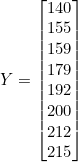
In matrix notation, the model is written as  . The four matrices are defined as follows.
The matrix ( ) — the dependent variable, quantity demanded:
The  matrix (
 ) — a column of 1’s (for the intercept), followed by income () and price ():
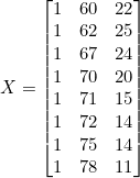
The  matrix (
 ) — the unknown population parameters to be estimated:

The error matrix () — the disturbance term for each observation:
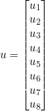
The complete model in matrix form is therefore , and OLS estimation gives us the sample counterpart  , where
  is the OLS coefficient vector and
  is the residual vector.
Step 3: Computing 
The transpose  is a
is a  matrix:
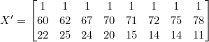
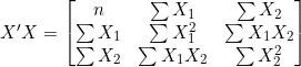
Multiplying  gives a symmetric
  matrix built from the sums
  ,
,  ,
,  ,
,  ,
,  , and
, and  :
:
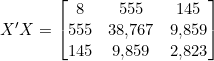
From the data:  ,
,  ,
,  ,
,  , and
, and  . So:
. So:
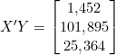
Step 4: Computing 
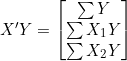
Multiplying  gives a
  vector built from
  ,
,  , and
, and  :
:
From the data:  ,
,  , and
, and  . So:
. So:
Step 5: Finding 
Determinant of (cofactor expansion along the first row):




So  .
.
Cofactors of :

![C_{12} = -[(555)(2{,}823) - (9{,}859)(145)] = -137{,}210](https://minhajmetrixhub.com/wp-content/ql-cache/quicklatex.com-f2473be087737281b77f522f18abbbc7_l3.png "Rendered by QuickLaTeX.com")


![C_{23} = -[(8)(9{,}859) - (145)(555)] = 1{,}603](https://minhajmetrixhub.com/wp-content/ql-cache/quicklatex.com-2d9eca4745d10e00ffa803366b904567_l3.png "Rendered by QuickLaTeX.com")

Since is symmetric, its cofactor (and adjugate) matrix is also symmetric. The inverse is  :
:


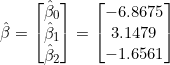
Step 6: Solving for the Coefficient Vector 

Using the exact integer numerators over the common determinant  (to avoid rounding error), each element of is found as the dot product of a row of the adjugate matrix with :



So the estimated coefficient vector is:
Step 7: The Estimated Regression Equation

This says that, holding price constant, a one-unit increase in income raises quantity demanded by about 3.15 units, while holding income constant, a one-unit increase in price reduces quantity demanded by about 1.66 units — both consistent with standard demand theory (a normal good with a downward-sloping demand curve).
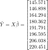
Step 8: Finding the Predicted Values 

Each predicted value is the dot product of a row of with , i.e.  :
:








So the predicted values matrix is:
Step 9: Finding the Residual Matrix 

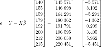
The residual vector is obtained by subtracting the predicted values matrix (Step 8) from the actual matrix, element by element:
| Obs. | |  |  |  |
|---|---|---|---|---|
| 1 | 140 | 145.571 | -5.571 | 31.04 |
| 2 | 155 | 146.898 | 8.102 | 65.64 |
| 3 | 159 | 164.294 | -5.294 | 28.03 |
| 4 | 179 | 180.362 | -1.362 | 1.86 |
| 5 | 192 | 191.791 | 0.209 | 0.04 |
| 6 | 200 | 196.595 | 3.405 | 11.59 |
| 7 | 212 | 206.038 | 5.962 | 35.54 |
| 8 | 215 | 220.451 | -5.451 | 29.71 |
The residuals sum to approximately zero ( ), confirming the OLS property that
  whenever an intercept is included.
Step 10: Residual Sum of Squares (RSS) via Matrices
Direct method: 
Matrix shortcut:  . First find
  :
:

Next,  :
:


Both approaches agree:  .
.
Step 11: Total Sum of Squares (TSS) via Matrices
 , where
  .
.


Step 12: Finding  Using Matrices
With  and
and  already obtained purely from matrix operations, follows directly:

This means 96.26% of the variation in quantity demanded is jointly explained by income and price, indicating a very good fit.
Step 13: Variance and the Variance-Covariance Matrix of 
The estimated variance of the error term is:

The variance-covariance matrix of the coefficient vector is  :
:
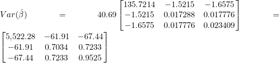
The standard errors of the coefficients are the square roots of the diagonal elements:



Step 14: t-Values and Tests of Significance
Each t-statistic is computed as 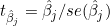 , with
  degrees of freedom:

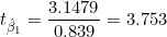

The critical t-value at the 5% level of significance (two-tailed,  ) is
) is  , and at the 10% level it is
  .
.
Interpretation
Intercept ( ):
):  , so the intercept is statistically insignificant. This is not unusual, since the intercept has no direct economic meaning here (income and price are never realistically zero).
Income coefficient ( ):
):  , so income is statistically significant at the 5% level. Higher consumer income significantly raises quantity demanded, as expected for a normal good.
Price coefficient ( ):
):  , so price is not significant at the conventional 5% two-tailed level. However, economic theory strongly predicts a negative price effect, which justifies a one-tailed test. The one-tailed 10% critical value at is
  ; since
  , the price effect is significant at the 10% level (one-tailed), though it remains a weaker result than the income effect.
Step 15: Income and Price Elasticity of Demand
Elasticities are calculated at the mean values of the variables, using  ,
,  , and
, and  .
.
Income elasticity of demand:

Since  , demand is income-elastic—the commodity behaves like a luxury good, with quantity demanded rising in proportion to income.
Price elasticity of demand:

Since  , demand is price-inelastic — a 1% increase in price reduces quantity demanded by only about 0.165%, suggesting the commodity has few close substitutes or is a necessity.
Regression Results (Academic / Research Paper Format)
The estimated demand function, with standard errors in parentheses and t-statistics in brackets below each coefficient, is reported as follows:



Table 1. OLS Estimates of the Demand Function
| Variable | Coefficient | Std. Error | t-Statistic | Significance (5%) |
|---|---|---|---|---|
| Intercept | -6.8675 | 74.312 | -0.092 | Not significant |
| Income () | 3.1479 | 0.839 | 3.753 | Significant |
| Price () | -1.6561 | 0.976 | -1.697 | Not sig. at 5% (two-tailed); sig. at 10% (one-tailed) |
Note:  ; ; degrees of freedom
  . Income elasticity of demand
  ; price elasticity of demand
  .
.
Overall Interpretation of the Model
The estimated model shows that consumer income and commodity price jointly explain about 96.26% of the variation in quantity demanded (), indicating a strong overall fit.
Income has a positive and statistically significant effect on demand, consistent with the good being a normal good; in fact, with an income elasticity greater than one, it behaves as a luxury good.
Price has the theoretically expected negative sign, but its effect is only marginally significant at conventional levels, and demand is price-inelastic, implying that consumers do not adjust their purchases much in response to price changes, possibly because the good has few substitutes or is a routine purchase.
The intercept itself is not economically meaningful and is statistically insignificant, which is expected since income and price are never realistically zero in practice.
Frequently Asked Questions
Q1: Why do we still add a column of 1’s in the X matrix for multiple regression?
Just as in simple regression, the column of 1’s lets matrix multiplication generate the intercept automatically, alongside the slope coefficients for each explanatory variable.
Q2: How is  found for a
  matrix?
It is found using the cofactor/adjugate method: compute the determinant via cofactor expansion, find the cofactor for each element, arrange them into the adjugate matrix (transpose of the cofactor matrix), and divide every element by the determinant.
Q3: Why is the intercept insignificant while income is significant?
The intercept represents the predicted value of when both and are zero — a scenario with no real-world meaning here, so it is common for the intercept’s t-value to be small and statistically insignificant. Income, by contrast, has direct economic relevance to demand and shows a strong, significant relationship.
Q4: What does an income elasticity greater than 1 tell us?
An income elasticity above 1 (here, 1.20) means the commodity is a luxury good — demand grows proportionally faster than income. Elasticity between 0 and 1 would indicate a normal necessity good, and a negative value would indicate an inferior good.
Q5: Why might price be statistically insignificant even though its coefficient has the expected negative sign?
With a small sample ( ) and a low price elasticity (demand is inelastic), the standard error on the price coefficient can be large relative to its estimate, reducing the t-value. This doesn’t necessarily mean price has no effect — it may reflect limited sample size or genuinely weak price sensitivity for this commodity.




 MinhajMetricsHub