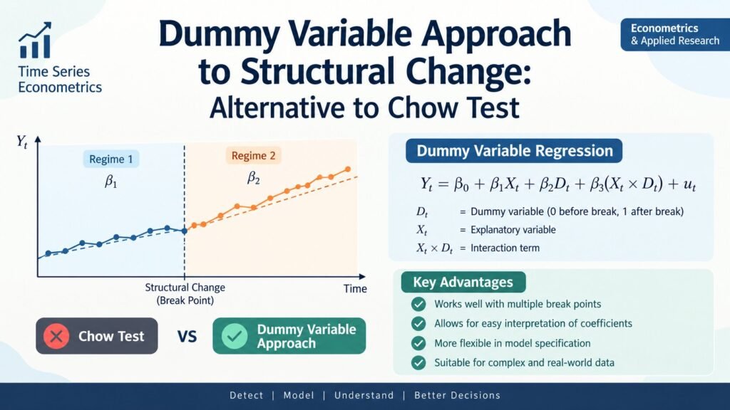
Dummy Variable Approach to Structural Change: Alternative to Chow Test

In the previous article, we used the Chow test to check whether the savings-income relationship for the US broke down after the 1982 recession, and we found that it did. But the Chow test left us with an unsatisfying answer.

It told us that the two regressions, 1970-1981 and 1982-1995, were significantly different, yet it could not tell us why. Was it the intercept that shifted, the slope, or both? The Chow test is silent on this question, and it also requires us to run three separate regressions and to already know the exact point at which the break occurred.

This article shows how a single dummy variable regression model answers the same question, and more, in one step.

Why the Chow Test Is Not Enough

Recall that the Chow test works by comparing the restricted residual sum of squares, obtained from a single regression run over the entire period, with the unrestricted residual sum of squares, obtained by adding together the residual sums of squares from two sub-period regressions.

A large F-statistic tells us that pooling the data into one regression is not justified; that is, there is a structural change. However, this procedure has three limitations.

• It does not identify the source of the instability, since a rejection of the null hypothesis could be due to a shift in the intercept alone, a shift in the slope alone, or both.
• It requires the researcher to know the break point in advance.
• It requires estimating three separate regressions rather than one, which is computationally wasteful and statistically less efficient because splitting the sample reduces the degrees of freedom available for each sub-regression.

The dummy variable regression model overcomes the first and third of these limitations directly, and it does so within the same F-test framework that the Chow test uses, so no new statistical machinery is required.

The Logic of the Dummy Variable Model

Suppose, as before, we have annual data on personal savings, , and disposable income, , for the United States from 1970 to 1995, and we suspect that the 1982 recession changed the savings-income relationship. Instead of splitting the sample and running three regressions, we define a single dummy variable

for observations in 1982–1995, and for observations in 1970–1981

and estimate one combined regression that includes the dummy, the dummy interacted with income, and income itself

Here is the intercept of the pre-1982 regression, is the differential intercept coefficient, telling us how much the intercept changes in the post-1982 period, is the slope, or the marginal propensity to save, in the pre-1982 period, and is the differential slope coefficient, telling us how much the slope changes in the post-1982 period.

To see why this single equation reproduces both sub-period regressions, set , which gives the savings function for 1970-1981

and set , which gives the savings function for 1982-1995

So the single regression is mathematically equivalent to running the two sub-period regressions separately, except that now the difference between the two regressions is captured directly by the estimated coefficients and , along with their standard errors, so we can test their significance individually.

The Four Possible Outcomes

Once the combined regression is estimated, the pattern of significance among and tells us exactly what kind of structural change, if any, has occurred. There are four possibilities.

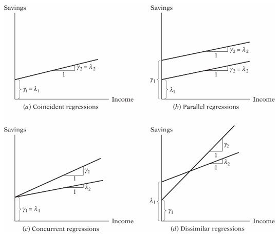
1. If both and are statistically insignificant, the two regression lines are essentially the same line. This is called a coincident regression, meaning there is no structural change at all.
2. If is significant but is not, only the intercept has shifted while the slope has stayed the same. The two regression lines are parallel to each other. This is called a parallel regression.
3. If is insignificant but is significant, the intercept has stayed the same but the slope has changed, so the two lines cross at the common intercept. This is called a concurrent regression.
4. If both and are significant, both the intercept and the slope differ between the two periods, and the lines are neither parallel nor coincident. This is called a dissimilar regression.

This classification is exactly the piece of information the Chow test cannot give us.

Testing Overall Stability

If we want a single test of whether the entire regression is stable, that is, whether simultaneously, we do not need a separate procedure. We simply run the usual restricted F-test, comparing the residual sum of squares of the restricted model, which drops and , with the residual sum of squares of the unrestricted model above.

This F-test is numerically identical to the Chow test, because the restricted model here is the same as the pooled regression in the Chow procedure, and the unrestricted model here has the same residual sum of squares as adding the two sub-period residual sums of squares.

So the dummy variable approach nests the Chow test as a special case while offering the additional diagnostic information the individual t-tests provide.

A Worked Example: US Personal Savings and Disposable Income, 1970-1995

Continuing with the same data used in the Chow test example, personal savings, , regressed on disposable income, , with the dummy equal to 1 for 1982-1995 and 0 for 1970-1981, suppose the estimated dummy variable regression is

with standard errors of 0.056, 0.512, 0.011 and 0.015 respectively, and corresponding t-ratios of approximately 5.75, 2.51, 7.09 and minus 2.73. With 22 degrees of freedom, the 5 percent critical t-value is close to 2.07, so all four coefficients are statistically significant, including both and .

Because both the differential intercept and the differential slope coefficients are significant, we conclude that this is a dissimilar regression, meaning both the intercept and the slope of the savings function changed after the 1982 recession. Substituting and gives us the two implied sub-period savings functions

for 1970–1981

for 1982–1995

The economic interpretation is straightforward. Before the 1982 recession, a one dollar increase in disposable income raised personal savings by about 7.8 cents, the marginal propensity to save. After the recession, this marginal propensity to save fell to about 3.7 cents, roughly half its earlier value, while the baseline level of savings, captured by the intercept, rose noticeably.

This pattern is consistent with a well documented feature of recessions, households increase precautionary savings at low levels of income right after the shock, but the sensitivity of savings to further increases in income weakens once income starts recovering, because consumption smoothing takes over.

If we now test the joint hypothesis using the restricted F-test described above, we obtain an F-statistic of 10.69 with 2 and 22 degrees of freedom, exactly the same value obtained from the Chow test in the previous article, with a p-value of 0.00057.

This confirms that the dummy variable regression and the Chow test agree on whether there is a structural change, but only the dummy variable regression tells us that the change is due to both the intercept and the slope.

Advantages of the Dummy Variable Approach Over the Chow Test

Only a single regression needs to be estimated, rather than three separate regressions, which is more convenient and uses the full sample when estimating the error variance.

Because all the observations are pooled into one regression, the degrees of freedom are higher, which improves the precision of the estimated parameters.

A single regression can be used to test a variety of hypotheses at once, simply by looking at the significance of and individually or jointly.

Most importantly, the approach pinpoints the source of the structural change. It tells us not just whether the regressions differ, but whether the difference lies in the intercept, the slope, or both, something the Chow test can never do on its own.

Conclusion

The Chow test is a useful first step for detecting whether a structural change has occurred, but it stops there. The dummy variable regression model builds on the same F-test logic while going one step further, decomposing the change into an intercept effect and a slope effect within a single, more efficient regression.

In practice, most applied econometricians run the dummy variable regression directly rather than the three separate Chow test regressions, precisely because it delivers the same test of overall stability along with a much richer diagnosis of what changed and by how much.