Derivation of OLS Estimator in Matrix Form

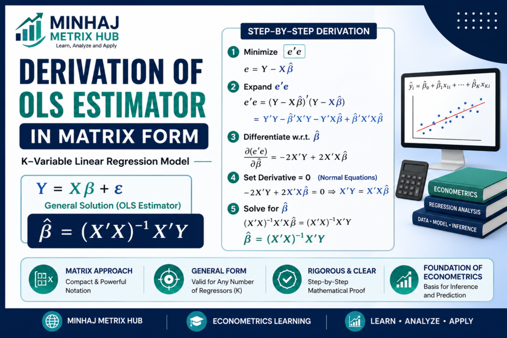
Matrix Approach to Linear Regression Model & Derivation of OLS Estimator in Matrix Form

Table of Contents

The K-Variable Linear Regression Model

Consider the following K-variable linear regression model:

$Y_i = \beta_0 + \beta_1 X_{i1} + \beta_2 X_{i2} + \cdots + \beta_K X_{iK} + \varepsilon_i$

Where εᵢ is the error term, it is distributed as normal with mean 0 (E(εᵢ) = 0) and variance σ² (Var(εᵢ) = σ², constant variance).

β₀, β₁, β₂, …, βK and σ² are true, unknown population parameters — β₀ is the intercept and β₁, …, βK are the partial slope coefficients on X₁, …, XK — estimated from sample data using an appropriate parameter-estimation method such as OLS or ML.

$\varepsilon_i \sim N(0,\sigma^2)$

Expanding the Model Across N Observations

Replacing the generic index i by 1, 2, 3, …, N produces N individual equations, one for each observation:

$Y_1 = \beta_0 + \beta_1 X_{11} + \beta_2 X_{12} + \cdots + \beta_K X_{1K} + \varepsilon_1$

$Y_2 = \beta_0 + \beta_1 X_{21} + \beta_2 X_{22} + \cdots + \beta_K X_{2K} + \varepsilon_2$

$\vdots$

$Y_N = \beta_0 + \beta_1 X_{N1} + \beta_2 X_{N2} + \cdots + \beta_K X_{NK} + \varepsilon_N$

or, for a representative observation i:

$Y_i = \beta_0 + \beta_1 X_{i1} + \beta_2 X_{i2} + \cdots + \beta_K X_{iK} + \varepsilon_i$

or, more compactly, in summation form:

$Y_i = \beta_0 + \sum_{j=1}^{K} \beta_j X_{ij} + \varepsilon_i$

The Model in Matrix Notation

We can now write the entire system of N equations compactly in matrix notation as:

$Y = X\beta + \varepsilon$

$\begin{array}{rcl} \begin{bmatrix} Y_1\\ Y_2\\ \vdots\\ Y_N \end{bmatrix} & = & \begin{bmatrix} 1 & X_{11} & X_{12} & \cdots & X_{1K}\\ 1 & X_{21} & X_{22} & \cdots & X_{2K}\\ \vdots & \vdots & \vdots & \ddots & \vdots\\ 1 & X_{N1} & X_{N2} & \cdots & X_{NK} \end{bmatrix} \begin{bmatrix} \beta_0\\ \beta_1\\ \vdots\\ \beta_K \end{bmatrix} \\ & & + \begin{bmatrix} \varepsilon_1\\ \varepsilon_2\\ \vdots\\ \varepsilon_N \end{bmatrix} \end{array}$

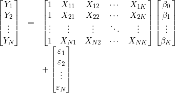
Equivalently, indicating the dimension (order) of every component:

$Y_{N\times1} = X_{N\times(K+1)}\,\beta_{(K+1)\times1} + \varepsilon_{N\times1}$

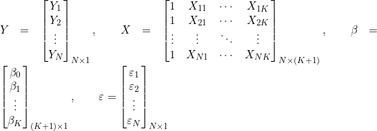
which is written as:

$Y = X\beta + \varepsilon$

Definitions and Dimensions of Each Component

Y = N × 1 column vector of values of the dependent variable.
X = N × (K + 1) matrix: a column of 1’s (for the intercept) plus K columns of explanatory variables X₁, X₂, …, X_K, across N observations.
β = (K + 1) × 1 column vector of (K + 1) unknown parameters (β₀ is the intercept; β₁, …, β_K are the slope coefficients).
ε = N × 1 column vector of N error terms.

Derivation of the OLS Estimator in Matrix Form

Overview

Building on the K-variable model introduced above, this lecture derives the Ordinary Least Squares (OLS) estimator $\hat{\beta}$ entirely in matrix notation — starting from the Population Regression Function (PRF), through minimization of the Sum of Squared Residuals (SSR), to the final closed-form solution. Every algebraic step—including two independent proofs of the matrix differentiation rules used—is shown explicitly.

The Population Regression Function (PRF) in Matrix Form

The Population Regression Function, written compactly in matrix form, is:

$Y = X\beta + \varepsilon,\qquad \varepsilon \sim N(0,\sigma^2)$

where the components are defined as follows:

Y is an N × 1 column vector of observations on the dependent variable.
X is an N × (K + 1) matrix — a column of 1’s for the intercept plus K explanatory variables X₁, …, XK — with N observations.
β is a (K + 1) × 1 column vector of (K + 1) unknown parameters (β₀ the intercept, and β₁,…,βK the slope coefficients).
ε is an N × 1 column vector of stochastic error terms, distributed as ε ~ N(0, σ²), with constant variance σ² (homoscedasticity).

$Y=\begin{bmatrix}Y_1\\Y_2\\\vdots\\Y_N\end{bmatrix}_{N\times1},\qquad X=\begin{bmatrix}1&X_{11}&\cdots&X_{1K}\\1&X_{21}&\cdots&X_{2K}\\\vdots&\vdots&\ddots&\vdots\\1&X_{N1}&\cdots&X_{NK}\end{bmatrix}_{N\times(K+1)},\qquad \beta=\begin{bmatrix}\beta_0\\\beta_1\\\vdots\\\beta_K\end{bmatrix}_{(K+1)\times1},\qquad \varepsilon=\begin{bmatrix}\varepsilon_1\\\varepsilon_2\\\vdots\\\varepsilon_N\end{bmatrix}_{N\times1}$

The Estimated (Sample) Regression Function

Because E(ε) = 0, the fitted (estimated) model is written as:

$\hat{Y}=X\hat{\beta}\qquad\text{[since }E(\varepsilon)=0\text{]}$

Objective: Minimizing the Sum of Squared Residuals (SSR)

The OLS estimator $\hat{\beta}$ is obtained by minimizing the Sum of Squared Residuals:

$\min \sum_{i=1}^{N} e_i^2=\sum_{i=1}^{N}(Y_i-\hat{Y}_i)^2$

Since Y is an N × 1 column vector, Ŷ must also be an N × 1 column vector, and their difference — the residual vector — is likewise N × 1:

$e_i=Y_i-\hat{Y}_i\qquad(N\times1\ \text{column vector})$

Expressing SSR in Matrix Notation

To obtain the sum of squared residuals, the residual vector (order N × 1) must be multiplied by its own transpose (order 1 × N). This product yields a scalar of order 1 × 1.

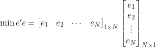
$\min e'e=\begin{bmatrix}e_1&e_2&\cdots&e_N\end{bmatrix}_{1\times N}\begin{bmatrix}e_1\\e_2\\\vdots\\e_N\end{bmatrix}_{N\times1}$

Thus, the minimization problem becomes:

$\min\sum_{i=1}^{N}e_i^2=e'e$

Expanding e′e

$e'e=(Y-\hat{Y})'(Y-\hat{Y})$

$e'e=(Y-X\hat{\beta})'(Y-X\hat{\beta})$

Applying the transpose rule (AB)′ = B′A′ to the first bracket:

$e'e=(Y'-\hat{\beta}'X')(Y-X\hat{\beta})\qquad[(AB)'=B'A']$

Distributing the second bracket across both terms:

$e'e=Y'(Y-X\hat{\beta})-\hat{\beta}'X'(Y-X\hat{\beta})$

Multiplying out fully gives the expanded quadratic form:

$e'e=Y'Y-Y'X\hat{\beta}-\hat{\beta}'X'Y+\hat{\beta}'X'X\hat{\beta}\qquad\cdots(1)$

Proving that Y′Xβ̂ is a Scalar

Checking the conformability and resulting dimension of the middle term:

$Y'_{1\times N}X_{N\times(K+1)}\hat{\beta}_{(K+1)\times1}=(Y'X)_{1\times(K+1)}\hat{\beta}_{(K+1)\times1}=(1\times1)_{\text{scalar}}$

Since $Y'X\hat{\beta}$ reduces to a 1 × 1 matrix, it is a scalar.

Simplifying via Transpose Property

The transpose of a scalar is the scalar itself. For example, if A = [5], then A′ = [5].

Taking the transpose of the scalar $Y'X\hat{\beta}$ and applying the rule (ABC)′ = C′B′A′:

$(Y'X\hat{\beta})'=\hat{\beta}'X'Y\qquad[(ABC)'=C'B'A]$

Since a scalar equals its own transpose, $Y'X\hat{\beta}=\hat{\beta}'X'Y$ . Substituting $\hat{\beta}'X'Y$ in place of $Y'X\hat{\beta}$ in equation (1) allows the two middle terms to be combined:

$e'e=Y'Y-2\hat{\beta}'X'Y+\hat{\beta}'X'X\hat{\beta}\qquad\cdots\ (2)$

First-Order Conditions: Differentiating e′e with respect to $\hat{\beta}$

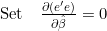
To minimize e′e, we differentiate equation (2) with respect to $\hat{\beta}$ and set the first derivative equal to the zero vector:

$\frac{\partial(e'e)}{\partial\hat{\beta}}=\frac{\partial}{\partial\hat{\beta}}(Y'Y)-2\frac{\partial}{\partial\hat{\beta}}(\hat{\beta}'X'Y)+\frac{\partial}{\partial\hat{\beta}}(\hat{\beta}'X'X\hat{\beta})$

The first term, $\frac{\partial}{\partial\hat{\beta}}(Y'Y)$ is zero since Y′Y does not depend on $\hat{\beta}$ . The remaining two derivatives are derived below with proof.

Derivative of the Linear Term $\hat{\beta}'X'Y$

Proof 1 — Element-wise expansion

Writing out the inner product explicitly (over all K + 1 parameters β̂₀, β̂₁, …, β̂K):

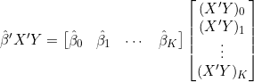
$\hat{\beta}'X'Y=\begin{bmatrix}\hat{\beta}_0&\hat{\beta}_1&\cdots&\hat{\beta}_K\end{bmatrix}\begin{bmatrix}(X'Y)_0\\(X'Y)_1\\\vdots\\(X'Y)_K\end{bmatrix}$

$\hat{\beta}'X'Y=\hat{\beta}_0(X'Y)_0+\hat{\beta}_1(X'Y)_1+\cdots+\hat{\beta}_K(X'Y)_K$

Taking partial derivatives with respect to each $\hat{\beta_i}$ and stacking them into a vector:

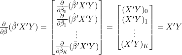
$\frac{\partial}{\partial\hat{\beta}}(\hat{\beta}'X'Y)=\begin{bmatrix}\frac{\partial}{\partial\hat{\beta}_0}(\hat{\beta}'X'Y)\\\frac{\partial}{\partial\hat{\beta}_1}(\hat{\beta}'X'Y)\\\vdots\\\frac{\partial}{\partial\hat{\beta}_K}(\hat{\beta}'X'Y)\end{bmatrix}=\begin{bmatrix}(X'Y)_0\\(X'Y)_1\\\vdots\\(X'Y)_K\end{bmatrix}=X'Y$

Proof 2—Matrix differentiation rule

Rule: $\frac{\partial}{\partial\hat{\beta}}(\hat{\beta}'c)=c$ , where c is a constant vector.

$\frac{\partial}{\partial\hat{\beta}}(\hat{\beta}'c)=c\qquad(c\text{ is a constant vector})$

Letting c = X′Y (a constant (K + 1) × 1 vector, since it does not depend on $\hat{\beta}$ :

$\text{Let }c=X'Y\;\Rightarrow\;\hat{\beta}'X'Y=\hat{\beta}'c\;\Rightarrow\;\frac{\partial}{\partial\hat{\beta}}(\hat{\beta}'X'Y)=X'Y$

Derivative of the Quadratic Term $\hat{\beta}'X'X\hat{\beta}$

The result of this derivative is:

$\frac{\partial}{\partial\hat{\beta}}(\hat{\beta}'X'X\hat{\beta})=2X'X\hat{\beta}$

Proof (using the matrix differentiation rule):

Rule: $\frac{\partial}{\partial\hat{\beta}}(\hat{\beta}'A\hat{\beta})=(A+A')\hat{\beta}$

$\text{Let }A=X'X,\quad\text{so}\quad\hat{\beta}'X'X\hat{\beta}=\hat{\beta}'A\hat{\beta}$

$\text{Rule:}\quad\frac{\partial}{\partial\hat{\beta}}(\hat{\beta}'A\hat{\beta})=(A+A')\hat{\beta}$

$\text{Since }X'X\text{ is symmetric:}\quad A'=(X'X)'=X'X=A$

$\therefore\quad\frac{\partial}{\partial\hat{\beta}}(\hat{\beta}'X'X\hat{\beta})=(A+A)\hat{\beta}=2A\hat{\beta}=2X'X\hat{\beta}$

Combining the Derivatives

Substituting both results back into the first-order condition:

$\frac{\partial(e'e)}{\partial\hat{\beta}}=-2X'Y+2X'X\hat{\beta}$

$\text{Set}\quad\frac{\partial(e'e)}{\partial\hat{\beta}}=0$

$-2X'Y+2X'X\hat{\beta}=0$

The Normal Equations

Solving the first-order condition for the stationary point:

$-2X'Y=-2X'X\hat{\beta}\;\Longrightarrow\;X'Y=X'X\hat{\beta}\qquad(\text{Normal Equations})$

This is the matrix form of the Normal Equations.

Solving for the OLS Estimator $\hat{\beta}$

Pre-multiplying both sides of the normal equations by the inverse (X′X)⁻¹:

$X'X\hat{\beta}=X'Y$

$\text{Pre-multiply both sides by }(X'X)^{-1}:$

$(X'X)^{-1}X'X\hat{\beta}=(X'X)^{-1}X'Y$

$I\hat{\beta}=(X'X)^{-1}X'Y$

which gives the OLS estimator in closed matrix form:

$\hat{\beta}=(X'X)^{-1}X'Y$

Condition for Existence of $\hat(\beta)$

$(X'X)^{-1}\text{ exists}\iff X\text{ has full column rank }(\operatorname{rank}(X)=K+1)$

If (X′X) is a non-singular (invertible) matrix, $\hat{\beta}$ can be uniquely determined. This inverse exists if and only if X has full column rank—that is, no explanatory variable (nor the intercept column) is an exact linear combination of the others (no perfect multicollinearity).

Summary: Key Steps

PRF: $Y=X\beta+\varepsilon$
Minimize SSR: $\min e'e=(Y-X\hat{\beta})'(Y-X\hat{\beta})$
Expand: $e'e=Y'Y-2\hat{\beta}'X'Y+\hat{\beta}'X'X\hat{\beta}$
Differentiate and set to zero: $-2X'Y+2X'X\hat{\beta}=0$
Normal equations: $X'Y=X'X\hat{\beta}$
Final Answer: $\hat{\beta}=(X'X)^{-1}X'Y$

Suggestions for further readings

About the author

Muhammad Minhaj Akhtar

Muhammad Minhaj Akhtar is a Lecturer in Economics at Government Graduate College Jauharabad, Pakistan. He holds an M.Phil. in Economics from Quaid-i-Azam University, Islamabad, and an MSc in Economics from the University of Sargodha, where he earned a Silver Medal. His academic passion lies in Econometrics, with a strong focus on applying empirical methods to real-world economic issues. Through MinhajMetrixHub, he shares learning resources, research guidance, and practical econometric insights for students and researchers.