The IS Curve Explained: Derivation, Slope, and Shift Factors

Macroeconomics studies how an entire economy behaves — how total output, the general price level, employment, and interest rates are determined. To understand these outcomes, economists typically divide the economy into three interconnected markets: the goods market, the money market, and the labour market. The famous IS-LM model, which we build up to in this article, is essentially a story about how the goods market and the money market interact to determine the interest rate and the level of national income in the short run.

Table of Contents

The Three Markets in Macroeconomics

Before deriving the IS curve, it is useful to understand where it fits within the broader structure of macroeconomic analysis.

The Goods Market

The goods market is where output — final goods and services — is produced, sold, and purchased. Equilibrium in this market occurs when the total output produced in the economy equals the total planned spending on that output (consumption, investment, and government spending). The IS curve, the subject of this article, describes all the combinations of the interest rate and national income at which the goods market is in equilibrium.

The Money Market

The money market is where the demand for and supply of money are balanced. The demand for money depends on income (people hold more money when their income is higher) and on the interest rate (money is held less when interest rates, and therefore the opportunity cost of holding money, are high). Equilibrium in this market is described by the LM curve, which is a separate topic from the one covered here.

The Labor Market

The labor market determines employment and, in many macroeconomic models, the price level and potential output through the interaction of labor demand and labor supply. While the IS-LM framework itself largely holds the price level fixed in the short run, the labor market becomes central once we move to models of aggregate supply.

The IS curve concerns only the goods market. Combined with the LM curve (money market equilibrium), it allows us to jointly determine the equilibrium interest rate and the equilibrium level of national income. This article focuses entirely on building and understanding the IS side of that framework.

From the Keynesian Cross to the IS Curve

In the basic Keynesian Cross model, planned investment, $I$ , is treated as autonomous — a fixed amount that does not depend on the interest rate. In reality, firms plan their investment spending with the interest rate in mind, since borrowing becomes more costly when interest rates are high. To capture this relationship, planned investment is written as a function of the interest rate:

$I = I(r)$

Figure 1: The Investment Function

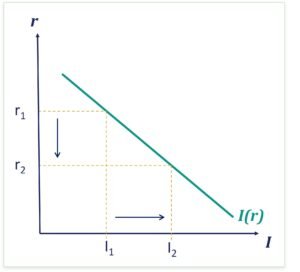
Because the interest rate is the cost of borrowing to finance investment projects, an increase in $r$ reduces planned investment. As the interest rate rises from $r_1$ to $r_2$ , investment falls from $I(r_1)$ to $I(r_2)$ . The investment function is therefore downward sloping when plotted against the interest rate.

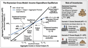
Since investment is a component of planned (aggregate) expenditure, and planned expenditure together with aggregate supply determines equilibrium output in the Keynesian Cross, a change in the interest rate—through its effect on investment—must also change equilibrium national income. This chain of reasoning, from the interest rate to investment to equilibrium output, is exactly what the IS curve captures.

What Is the IS Curve? Definition and Origin

The IS curve shows the various combinations of the interest rate and national income at which the goods market is in equilibrium.

The IS-LM model was developed by the economist John Richard Hicks in his 1937 paper, “Mr Keynes and the Classics”. It provided a graphical representation of the ideas in Keynes’s General Theory and became the standard tool for explaining short-run fluctuations in output and interest rates.

Together, the IS and LM curves determine the equilibrium interest rate and level of national income in the short run. The IS curve on its own is derived by combining the interest-sensitive investment function with the Keynesian Cross.

Graphical Derivation of the IS Curve

The IS curve can be derived graphically in four logical steps, moving from the investment function to the Keynesian Cross diagram and finally to the interest rate–income plane.

Step 1 — A change in the interest rate changes investment. An increase in the interest rate from $r_1$ to $r_2$ reduces the quantity of investment from $I(r_1)$ to $I(r_2)$ , because investment is inversely related to the interest rate.

Step 2 — The planned-expenditure line shifts. The reduction in planned investment shifts the planned-expenditure ( $AE$ ) function downward in the Keynesian Cross diagram, since investment is one component of total planned spending.

Step 3 — Equilibrium income falls. The downward shift in planned expenditure causes equilibrium income to fall from $Y_1$ to $Y_2$ , through the multiplier process along the 45-degree line of the Keynesian Cross.

Step 4 — Plotting the IS curve. Plotting each interest-rate/income pair, $(r_1, Y_1)$ and $(r_2, Y_2)$ , on a diagram with the interest rate on the vertical axis and income on the horizontal axis traces out the IS curve. Since a rise in $r$ lowers investment, which lowers equilibrium income, the IS curve slopes downward.

Figure 2: Derivation of IS Curve Using Keynesian Cross Diagram

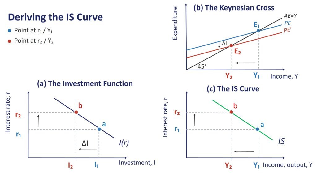
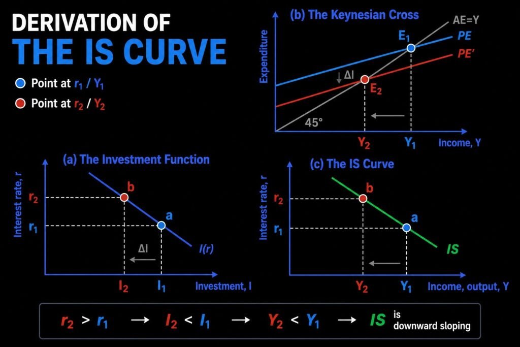
This logic is usually summarised using a three-panel diagram as shown in Figure 2: the first panel shows the investment function $I(r)$ , the second panel shows the Keynesian Cross with the 45-degree line, and the third panel plots the resulting interest-rate/income pairs to form the IS curve itself.

Reading down from the interest rate axis in panel I to the investment function gives the level of investment; that investment level shifts the expenditure line in panel II and determines equilibrium income; and each interest-rate/income combination is then plotted as a point in panel III. Joining all such points traces the downward-sloping IS curve.

Mathematical Derivation of the IS Curve

The graphical logic above can be formalised into a precise algebraic expression for the IS curve. We proceed step by step.

Step 1 — Goods-market equilibrium condition. Goods-market equilibrium requires that output equals planned expenditure, which consists of consumption, investment, and government spending:

$Y = C + I + G$

Step 2 — Behavioral equations. We specify each component of expenditure as a function of the relevant variables.

The consumption function is:

$C = C_0 + c(Y - T)$

where $C_0 > 0$ is autonomous consumption and $0 < c < 1$ is the marginal propensity to consume (MPC).

The investment function is:

$I = I_0 - er$

where $I_0 > 0$ is autonomous investment and $e > 0$ measures the interest-sensitivity of investment.

Fiscal policy is treated as exogenous (fixed by policy):

$G = G_0 \quad \text{and} \quad T = T_0$

Step 3 — Substitute the behavioral equations into the equilibrium condition.

$Y = C_0 + c(Y - T_0) + (I_0 - er) + G_0$

Expanding the bracket:

$Y = C_0 + cY - cT_0 + I_0 - er + G_0$

Step 4 — Collect all income terms on one side.

$Y - cY = C_0 + I_0 + G_0 - cT_0 - er$

Factoring out $Y$ on the left-hand side:

$Y(1 - c) = C_0 + I_0 + G_0 - cT_0 - er$

Step 5 — Solve for the interest rate. Rearranging to isolate the term containing $r$ :

$er = C_0 + I_0 + G_0 - cT_0 - Y(1 - c)$

Dividing both sides by $e$ gives the IS equation in its explicit form:

$r = \frac{C_0 + I_0 + G_0 - cT_0 - Y(1 - c)}{e}$

This single equation is the algebraic statement of the IS curve — it gives every combination of $r$ and $Y$ at which the goods market clears, for given values of autonomous spending, the MPC, government spending, and taxes.

Slope of the IS Curve

It is useful to rewrite the IS equation in a standard linear form, $r = \alpha_{IS} - \beta_{IS} Y$ is not quite the convention used here — instead, economists usually write it as:

$r = \alpha_{IS} + \beta_{IS} Y$

where the intercept and slope are:

$\alpha_{IS} = \frac{C_0 + I_0 + G_0 - cT_0}{e}$

$\beta_{IS} = \frac{dr}{dY} = -\frac{(1 - c)}{e}$

Since $0 < c < 1$ and $e > 0$ , the slope $\beta_{IS}$ is always negative. This confirms algebraically what the graphical derivation already showed: the IS curve is downward sloping. Any change in $G$ , $T$ , $C_0$ , or $I_0$ changes the intercept $\alpha_{IS}$ and therefore shifts the whole curve, while a change in $Y$ simply represents a movement along the given curve.

The steepness of the IS curve — how flat or steep it is — depends on two factors: the elasticity of investment demand with respect to the interest rate, and the size of the multiplier (which depends on the MPC).

Elasticity of Investment Demand

The elasticity of investment demand measures how responsive investment spending is to a given change in the interest rate. This is captured by the parameter $e$ in the investment function.

High elasticity (large $e$ ) → Flatter IS curve. A given rise in the interest rate causes a large decrease in investment. This large fall in investment brings about a large decrease in national income, so the IS curve is flatter.
Low elasticity (small $e$ ) → Steeper IS curve. A given rise in the interest rate causes only a small decrease in investment. The small fall in investment brings about only a small decrease in national income, so the IS curve is steeper.

The Multiplier and the MPC

The second determinant of slope is the size of the expenditure multiplier, $\dfrac{1}{1-c}$ , which itself depends on the marginal propensity to consume.

Higher MPC → Flatter IS curve. A greater MPC makes the aggregate-expenditure line steeper and the multiplier larger. A given fall in the interest rate then brings about a large increase in investment and, through the multiplier, an even larger increase in equilibrium national income — so the IS curve is flatter.
Lower MPC → Steeper IS curve. A smaller MPC means a smaller multiplier. A given fall in the interest rate brings about only a small increase in investment and equilibrium income, so the IS curve is steeper.

Formally, the magnitude of the slope is $\left| \dfrac{dr}{dY} \right| = \dfrac{1-c}{e}$ , which can also be written as 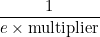$\dfrac{1}{e \times \text{multiplier}}$ . A larger multiplier (from a higher MPC) or a larger interest-sensitivity of investment ( $e$ ) both reduce the magnitude of the slope — that is, they flatten the IS curve.

Shift Factors of the IS Curve

The IS curve is drawn for a given level of autonomous expenditure and a given fiscal policy. The position of the entire curve — as opposed to movement along a given curve — depends on the level of autonomous expenditure: spending that does not depend on the level of national income, such as autonomous investment, autonomous government spending, and autonomous consumption. Any change in these components shifts the IS curve. The three main shift factors are autonomous investment, government spending, and taxes.

Government Spending

An increase in government spending by $\Delta G$ , holding the interest rate $\bar{r}$ and planned investment fixed, shifts the planned-expenditure curve upward. Equilibrium national income rises by $\Delta G$ times the government-spending multiplier:

$\Delta Y = \Delta G \times \frac{1}{1 - c}$

For a given interest rate, this means the IS curve shifts rightward.

Taxes

A reduction in taxes raises disposable income and therefore consumption, shifting the planned-expenditure curve rightward. Equilibrium income rises by $\Delta T$ times the tax multiplier:

$\Delta Y = \Delta T \times \left( \frac{-c}{1 - c} \right)$

Since a fall in $T$ (a negative $\Delta T$ ) produces a positive $\Delta Y$ , a tax cut shifts the IS curve rightward as well.

Autonomous Investment

Given the interest rate $\bar{r}$ , an increase in the expected profitability of investment raises investment expenditure and shifts the planned-expenditure curve upward. This raises equilibrium national income by:

$\Delta Y = \frac{\Delta I}{1 - c}$

This shifts the IS curve to the right at every given interest rate. The same logic applies in reverse: a fall in expected profitability, a fall in government spending, or a rise in taxes shifts the IS curve leftward.

Summary

The IS curve shows the combinations of the interest rate and the level of income at which the goods market is in equilibrium.
It is derived by combining the interest-sensitive investment function, $I(r)$ , with the Keynesian Cross, and it slopes downward because a rise in the interest rate lowers investment, which in turn lowers equilibrium income.
Its slope is flatter when investment demand is more elastic with respect to the interest rate, and when the MPC — and hence the multiplier — is larger.
It is drawn for a given fiscal policy ( $G$ and $T$ ) and given autonomous spending. Policies or changes that raise demand for goods and services (higher $G$ , lower $T$ , higher autonomous investment) shift the IS curve rightward; those that reduce demand shift it leftward.

Share this article

About the author

Muhammad Minhaj Akhtar

Muhammad Minhaj Akhtar is a Lecturer in Economics at Government Graduate College Jauharabad, Pakistan. He holds an M.Phil. in Economics from Quaid-i-Azam University, Islamabad, and an MSc in Economics from the University of Sargodha, where he earned a Silver Medal. His academic passion lies in Econometrics, with a strong focus on applying empirical methods to real-world economic issues. Through MinhajMetrixHub, he shares learning resources, research guidance, and practical econometric insights for students and researchers.