Life Cycle Hypothesis of Consumption: 3 Stages of Life Explained

Table of Contents

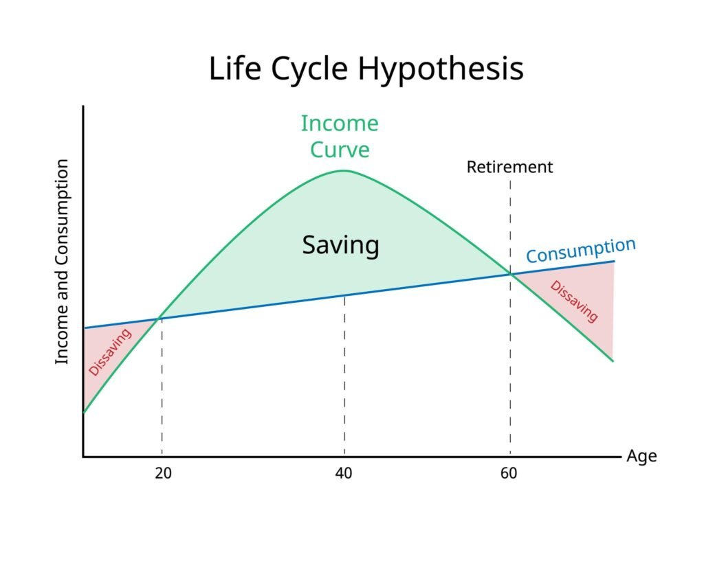
The Life Cycle Hypothesis of Consumption:

How Modigliani and Ando Explained a Lifetime of Spending

Why does a young graduate happily spend more than she earns, while a fifty-year-old professional saves carefully, only to spend those same savings twenty years later? Simple Keynesian theory, which links spending only to the current year’s income, cannot explain this pattern.

Franco Modigliani and Albert Ando, writing in the American Economic Review in March 1963, offered a different view. They argued that people do not decide how much to spend based on the current year’s income alone. Instead, they plan their spending over their whole life. This idea is known as the Life Cycle Hypothesis.

From Keynes to Modigliani: How the Theory Developed

The Life Cycle Hypothesis (LCH) did not appear on its own. It was the fifth major theory in a series of ideas that tried to explain how people decide how much to spend and how much to save.

John Maynard Keynes, in his Absolute Income Hypothesis, was the first to study this question closely. He said that spending depends on current income and that the share of income spent falls as income rises.

Later, Simon Kuznets’ consumption study on the US economy looked at long-run data and found something different: over long periods, the share of income spent stayed fairly stable. This went against what Keynes had predicted.

James Duesenberry in his Relative Income Hypothesis, said that spending depends on how a person’s income compares to other people’s income and to their own past highest income. After him, Milton Friedman introduced the Permanent Income Hypothesis. He argued that people base their spending on their permanent, long-term income, not on short-term ups and downs.

Modigliani and Ando built on all of these ideas. But instead of looking at income year by year, they looked at income and spending across a person’s entire life.

The Main Idea: Spreading Spending Across a Lifetime

The main idea of the Life Cycle Hypothesis is that consumption expenditure in any single year is not based only on that year’s income. Instead, it depends on how much a person expects to earn over their whole life and on how much wealth they already have. Thus, consumption depends on whole life income and wealth.

According to Modigliani and Ando, people try to keep their spending fairly steady, or slowly rising, across their whole life. In simple terms, people spread out their spending: they borrow when they are young, save during their working years, and use up their savings after they retire.

Key Assumptions of the Theory

Like most economic models, the Life Cycle Hypothesis is built on a few simple assumptions:

A fixed lifespan: the person is assumed to know exactly how long they will live.
Planning for the whole life: spending decisions are made all at once, based on income expected over the person’s entire life.
Steady spending: the person keeps a roughly equal, or slowly rising, level of spending throughout life.
Starting work at 15: The person is assumed to begin working and earning income at age 15.
Stable prices: prices are assumed to stay the same throughout a person’s life.
No plan to leave money behind: total savings equal zero by the end of life, so the person dies with no assets left.
No interest earned: to keep things simple, any interest earned on savings is assumed to be zero.
No pension: after retiring, the person is assumed to receive no pension or government support.

The Three Stages of Life

Modigliani and Ando divide a person’s economic life into three stages. In each stage, the relationship between income and spending is different.

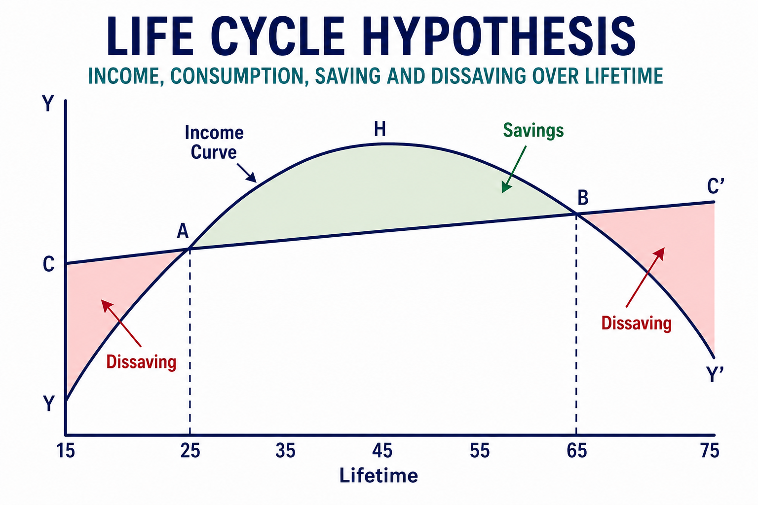
Figure 1: Life Cycle Hypothesis of Consumption

1. Early Age (about 15–25 years)

In his early or young age, a person spends more than he earns. This is called net dissaving. The gap is covered either by borrowing or by using money left by parents. Even though income slowly rises during this stage, it remains below the level of spending until approximately age 25 (referred to as Point A), when income finally catches up and equals consumption.

2. Middle / Working Age (about 25–65 years)

The person now spends less than she earns. From Point A (age 25) to Point B (age 65), income is higher than spending every year, so the person saves money. These savings build up as wealth. This wealth does two things: it pays off the debt taken on during the early years, and it builds a reserve to cover spending after retirement, when income will fall again.

3. Old Age / Retirement (about 65–75 years)

The person spends more than she earns again. After Point B, income drops well below the level of spending, so the person dissaves once more — this time by using up saved wealth instead of borrowing.

Since the model assumes no plan to leave money behind, total wealth returns to zero by the end of the expected life (age 75). If a person does want to leave money to their children, this assumption changes: they must save more during their working years, so total savings become larger than total dissaving.

Across all three stages, the person spreads out their spending. They save in the years when income is high and dissave in the years when income is low.

The Life Cycle Consumption Function

According to the Life Cycle Hypothesis, a person’s spending depends not just on current income but on total lifetime resources. These resources include starting wealth bequeathed by her parents, $W$ , plus total future labour income, $R \times Y$ , where $R$ is the number of years left before retirement and $Y$ is yearly labour income.

To keep spending steady, the person divides these total resources $(W + RY)$ equally across the $T$ years they expect to live. So each year, the person spends:

$C = \frac{W + RY}{T}$

Where:

$C$ — spending (consumption)
$W$ — starting wealth
$R$ — years left before retirement
$Y$ — yearly labour income
$RY$ — total future labour income
$T$ — years the person expects to live
$1/T$ — the fixed share of total resources spent each year

A Simple Example

Suppose a person expects to live for 50 more years, so $T = 50$ , and expects to work for 30 more of those years, so $R = 30$ . The spending equation becomes:

$C = \frac{1}{50}W + \frac{30}{50}Y = 0.02W + 0.6Y$

This equation shows that spending depends on both income and wealth. An extra dollar of yearly income raises spending by $0.60 per year. An extra dollar of wealth raises spending by only$ 0.02 per year.

The Aggregate Consumption Function

When we look at the whole economy together, the Life Cycle aggregate Consumption Function is usually written as the following:

$C = \alpha W + \beta Y$

Here, $\alpha$ is the share of extra wealth that goes toward spending, and $\beta$ is the share of extra income that goes toward spending.

Average Propensity to Consume: Linking Keynes and Kuznets

If we divide the aggregate spending equation by income, we get the average propensity to consume (APC) — the share of income that is spent:

$APC = \frac{C}{Y} = \alpha \frac{W}{Y} + \beta$

This one equation helps explain two findings that once looked contradictory.

In the short run, wealth does not rise at the same speed as income. So when income rises quickly, the ratio $W/Y$ falls, and the APC falls with it — just as Keynes had observed.
But over a long period, wealth and income tend to rise together. This keeps $W/Y$ roughly steady, which keeps the APC roughly steady too — just as Kuznets had observed.

In this way, the Life Cycle Hypothesis shows that Keynes and Kuznets were not really disagreeing. They were simply looking at different time periods within the same overall pattern.

Short-Run and Long-Run Consumption Functions

This idea is often shown on a graph as a set of short-run spending lines (SR1, SR2, SR3) that move upward over time. Together, these short-run lines trace out one long-run spending line (LRCF).

Figure 2: Short Run and Long Run Consumption Functions

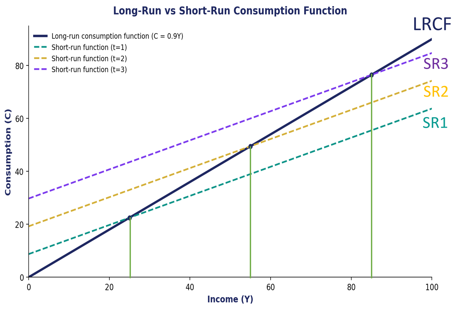
Each short-run line has a fixed starting point, which depends on the level of wealth at that time. Its slope shows how much extra spending comes from an extra dollar of current income. Because this starting point is above zero, the APC falls as income rises along any single short-run line, and the MPC remains lower than the APC

As a person’s wealth grows during their working years, the whole short-run line shifts upward. If we mark the points where each short-run line matches the person’s actual income and wealth at that time, we get the long-run spending line. Because it reflects the steady growth of both wealth and income together, this long-run line passes through origin.

Spending, Income, and Wealth Over the Life Cycle

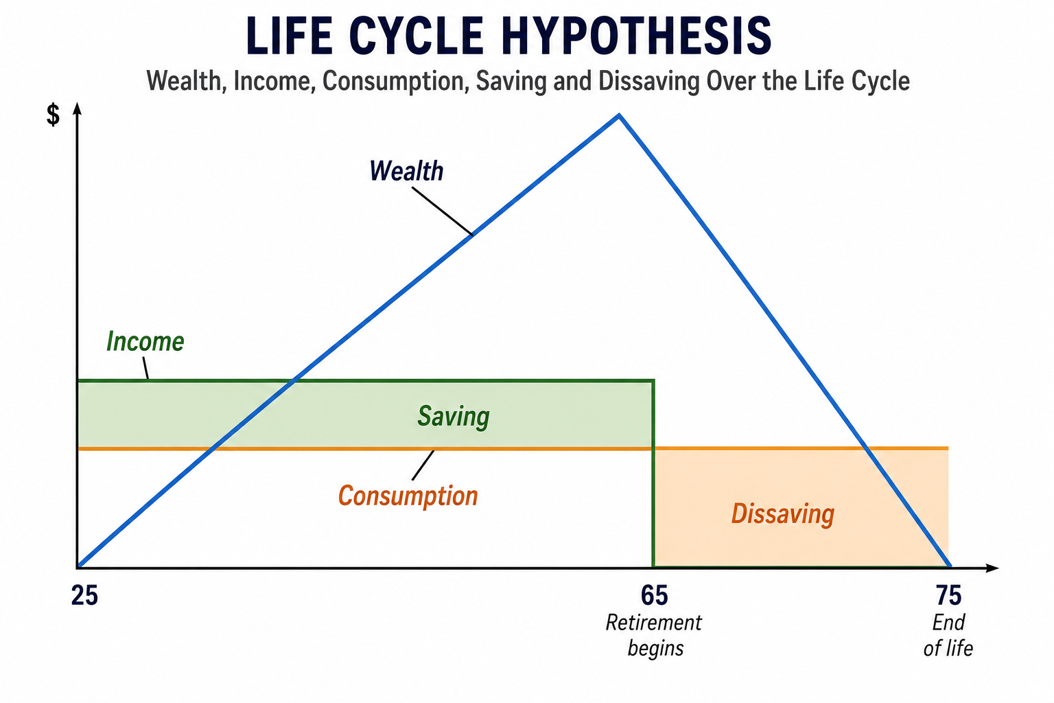
Plotting spending, income, and wealth together over a person’s life shows how this spreading-out process works. If a person keeps their spending fairly steady — shown as a flat line on the graph — they will save and build up wealth during their working years and then use up that wealth during retirement. As a result, wealth itself rises through the middle years of life and falls again after retirement, forming a rounded, hill-shaped pattern over the whole lifetime.

Figure 3: Spending, Income, and Wealth Over the Life Cycle

Criticisms of the Life Cycle Hypothesis

Despite its clear and simple structure, the Life Cycle Hypothesis has faced strong criticism, mostly aimed at its assumptions:

It assumes people can predict their future income almost perfectly. In real life, this is very hard to do.
It assumes people can borrow freely when they are young. In practice, banks are often careful about lending, and credit is not always easy to get.
It assumes people spend all their savings by the end of life. But many people want to leave money for their children.
It does not fully consider that people usually do not know exactly how long they will live.
Government pensions and old-age support can change how much people feel they need to save on their own. The basic model leaves this out.
Measuring “wealth” and “expected future income” in real data is genuinely difficult, which makes the theory hard to test.
The theory largely ignores habits and psychology. Many people simply spend based on today’s income, rather than planning across their whole life.

Economist Gardner Ackley, among others, pointed out that the assumption of near-perfect foresight is especially unrealistic. The theory’s lack of attention to borrowing limits is also one of its most commonly cited weaknesses.

Key Takeaways

Spending is planned over the whole life, based on expected lifetime income and wealth — not just current income.
People move through three stages of life: dissaving in youth, saving during working years, and dissaving again in retirement.
Current income raises spending sharply mainly when it also changes what a person expects to earn in the future. Changes in wealth shift the starting point of the spending line, not its slope.
The theory brings together Keynes’s short-run findings and Kuznets’s long-run findings within one framework.
It explains why high-income, middle-aged households tend to save more than low-income, young, or retired households.
Its main weaknesses are its assumption of near-perfect foresight and its failure to account for real-world limits on borrowing.

Conclusion

The Life Cycle Hypothesis marked an important shift in how economists think about spending. Instead of treating each year’s spending as a separate reaction to that year’s income, Modigliani and Ando pictured households as forward-looking planners, spreading their resources across a whole lifetime. This one change in perspective helped bring together the short-run and long-run findings that had once divided Keynes and Kuznets. The theory still shapes how economists study saving behaviour, retirement planning, and wealth today, even though its assumptions about perfect foresight and easy borrowing continue to draw fair criticism.

This lecture note is part of an ongoing intermediate macroeconomics series on Minhaj Metrix Hub, covering the development of consumption theory from Keynes through Modigliani and Ando’s Life Cycle Hypothesis.

Suggestions for further readings.

About the author

Muhammad Minhaj Akhtar

Muhammad Minhaj Akhtar is a Lecturer in Economics at Government Graduate College Jauharabad, Pakistan. He holds an M.Phil. in Economics from Quaid-i-Azam University, Islamabad, and an MSc in Economics from the University of Sargodha, where he earned a Silver Medal. His academic passion lies in Econometrics, with a strong focus on applying empirical methods to real-world economic issues. Through MinhajMetrixHub, he shares learning resources, research guidance, and practical econometric insights for students and researchers.