Keynesian Cross Model: Equilibrium of National Income Explained

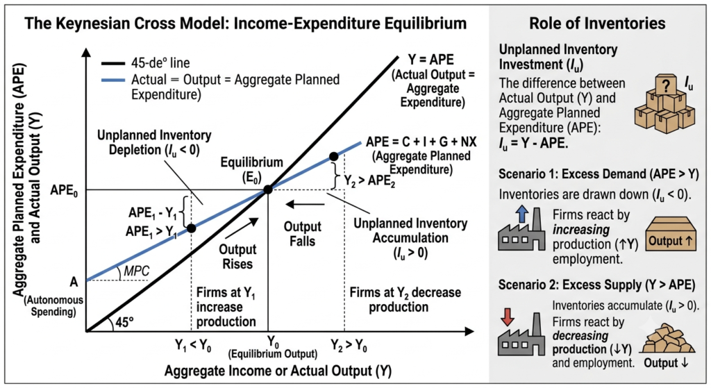
Why does an economy sometimes get stuck producing less than it could, with willing workers and idle machines sitting unused? Classical economists assumed markets would sort this out through prices and wages. Keynes argued something more powerful: output is driven by aggregate demand, and the economy can settle into equilibrium well below full employment. The Keynesian Cross model is the simplest, clearest way to see this argument at work, and it is the essential first step toward the more complete IS–LM framework.

This post builds the model from the ground up for a three-sector (closed) economy — households, firms, and government, with no foreign sector — and works through the assumptions, the graphical picture, the inventory-adjustment story, and a full algebraic derivation of equilibrium national income, with two worked numerical examples.

Table of Contents

The Three-Sector Economy

A three-sector economy has three spending units, and because there is no foreign sector, exports and imports are excluded entirely:

Households (H) — consume goods and services ( $C$ ), supply labour, and pay taxes ( $T$ )
Business firms (F) — undertake investment spending ( $I$ ), produce output, and hire factors of production
Government (G) — spends on goods and services ( $G$ ) and collects taxes ( $T$ )

Total planned spending in this economy is simply $C + I + G$ . Everything that follows is about how this spending interacts with output to determine where the economy settles.

Actual Expenditure vs. Planned Expenditure: A Crucial Distinction

Before we can define equilibrium, we need to separate two ideas that look similar but are not the same.

Actual Expenditure (AE) is what was really spent by households, firms, and governments on domestically produced goods and services. It always includes any unplanned change in business inventories.

This is why the following is an accounting identity — it holds whether or not the economy is in equilibrium:

$Y \equiv C + I + G \equiv AE$

The logic is simple: any output a firm produces but does not sell is not lost — it is added to inventories, and that addition is itself counted as investment spending. So whatever is produced is, by definition, also “spent” in this broad sense. Actual expenditure can never diverge from output.

Planned Expenditure (PE), also called desired or intended expenditure, is different. It is what households, firms, and governments intend to spend, an ex-ante concept that excludes unplanned inventory changes:

$PE = C + I + G$

Notice the two equations look alike, but $I$ means something different in each: in the AE identity, $I$ includes unplanned inventory changes; in the PE relationship, $I$ is only the planned (desired) investment. Planned expenditure equals national income only when the economy happens to be at equilibrium — it is a behavioural relationship, not an identity.

Feature	Actual Expenditure (AE)	Planned Expenditure (PE)
Nature	Realised, ex-post	Intended, ex-ante
Inventories	Includes unplanned changes	Excludes unplanned changes
Relation to Y	Always equal to Y (identity)	Equal to Y only at equilibrium
Can it diverge from output?	Never	Yes, whenever the economy is off equilibrium

Assumptions of the Keynesian Cross Model

Like any model, the Keynesian Cross simplifies reality to isolate one mechanism — the link between spending and output. It rests on the following assumptions:

Fixed price level. The analysis is short-run: prices and wages are assumed constant, so any change in demand shows up as a change in output, not in prices.
Autonomous investment. Planned investment, $I_0$ , is treated as exogenously given — it does not depend on the current level of income (interest-rate effects are set aside until the IS–LM stage).
Fixed fiscal policy variables. Government spending $G_0$ and taxes $T_0$ are policy variables set from outside the model, independent of income.
A stable, linear consumption function. Consumption depends only on current disposable income, $C = C_0 + cY_d$ , with the marginal propensity to consume $c$ constant and $0 \lt c \lt 1$ .
A closed, three-sector economy. There is no foreign sector, so exports and imports are both zero.
Output can settle below full employment. Equilibrium simply means planned spending equals output — there is no requirement that this happen at full-employment income. This is the central Keynesian departure from the classical view.
Firms adjust quantities, not prices. When planned spending and output diverge, firms respond by changing production levels in response to unplanned inventory movements, rather than by changing prices.

Why the Keynesian Cross Model Matters

Despite its simplicity, this model does a lot of conceptual work:

It shows demand, not supply, drives short-run output. Equilibrium income is wherever planned spending puts it – it is not fixed by the economy’s productive capacity.
It explains the adjustment mechanism. Unplanned changes in business inventories are the signal that pushes output back toward equilibrium from either side.
It introduces the expenditure multiplier. A small change in autonomous spending produces a larger change in equilibrium income — one of the most important results in macroeconomics.
It is the basic tool for fiscal policy analysis. Changes in government spending or taxes can be traced through to their effect on national income directly from this framework.
It is the building block for the IS curve. Once the interest rate is allowed to affect investment, this same cross becomes the starting point for the IS–LM model of the goods and money markets together.

Components of Planned Expenditure

Planned expenditure in a three-sector economy has three behavioural pieces:

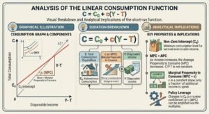
Consumption. Households spend a stable fraction of their disposable income, $Y_d = Y - T$ :

$C = C_0 + cY_d = C_0 + c(Y - T)$

Here $C_0$ is autonomous consumption (spending that would occur even at zero disposable income) and $c$ is the marginal propensity to consume — the fraction of each extra unit of disposable income that gets spent rather than saved.

Investment. In this basic model, planned investment is autonomous: $I = I_0$ , fixed independently of the current level of income.

Government. Government spending and taxes are both treated as policy-determined and fixed: $G = G_0$ and $T = T_0$ .

The Keynesian Cross Diagram

The Keynesian Cross is a simple graphical model that shows how planned expenditure and national income (output) interact to determine the equilibrium level of national income in the short run. It plots Planned Expenditure (PE) against National Income (Y), together with a 45° line representing every point where PE = Y.

Figure 1: The Keynesian Cross — the PE line cuts the 45° line at E, fixing equilibrium income at Y*.

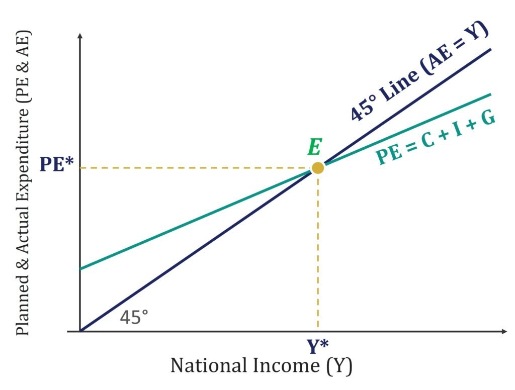
The diagram above plots planned expenditure on the vertical axis against national income on the horizontal axis, together with a 45° reference line along which every point satisfies $AE = Y$ . The PE line has a positive vertical intercept (autonomous spending, $A_0$ ) and a slope equal to the MPC, $c$ , which is less than 1 — planned spending rises with income, but by a smaller amount than income itself rises.

The equilibrium level of national income, $Y^*$ , occurs exactly where the PE line crosses the 45° line, at point $E$ . This is the equilibrium condition:

$PE = Y \quad \left(\text{equivalently } PE = AE, \text{ since } AE \equiv Y\right)$

At this single point, and only at this point, what firms plan to sell exactly matches what the economy produces.

The Role of Inventories in Restoring Equilibrium

What actually pulls the economy toward $Y^*$ when it starts somewhere else? The answer is unplanned changes in business inventories, and it is worth walking through both directions carefully.

Figure 1: Adjustment to Equilibrium in Keynesian Cross Diagram

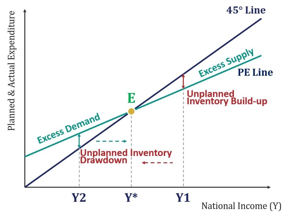
Case 1 — Output is above equilibrium ( $Y \gt Y^*$ ). At this income level the PE line lies below the 45° line, so $PE \lt Y$ : firms are producing more than households, businesses, and government plan to buy. The unsold output does not vanish — it piles up as an unplanned addition to inventories, above the level firms actually wanted to hold. Seeing inventories accumulate beyond their desired level, firms cut back production. Output, income, and employment all fall, and $Y$ moves down toward $Y^*$ .

Case 2 — Output is below equilibrium ( $Y \lt Y^*$ ). Here the PE line lies above the 45° line, so $PE \gt Y$ : there is excess demand. Firms meet this demand in the short run by selling out of existing inventories, so stocks fall below the desired level. To rebuild inventories and meet the demand they are seeing, firms raise production. Output, income, and employment all rise, and $Y$ moves up toward $Y^*$ .

At $Y = Y^*$ , planned expenditure exactly equals output, so there is no unplanned inventory change in either direction. Firms have no reason to raise or lower production — this is precisely why the point is stable. In short, unplanned inventory investment is the economy’s self-correcting signal: it is what firms actually observe and react to, quarter after quarter, in the absence of any change in prices.

Mathematical Derivation of Equilibrium National Income

Setting Up the Model

Collecting the behavioural equations for a three-sector economy:

$C = C_0 + c(Y - T_0)$

$I = I_0 \qquad G = G_0 \qquad T = T_0$

Substituting these into $PE = C + I + G$ :

$PE = \left[C_0 + c(Y - T_0)\right] + I_0 + G_0$

$PE = \left(C_0 - cT_0 + I_0 + G_0\right) + cY$

The bracketed term is total autonomous expenditure — everything in planned spending that does not depend on current income. Calling it $A_0 = C_0 - cT_0 + I_0 + G_0$ for convenience:

$PE = A_0 + cY$

Solving for Equilibrium Y

Impose the equilibrium condition, $Y = PE$ :

$Y = A_0 + cY$

$Y - cY = A_0$

$Y(1-c) = A_0$

$Y^{*} = \frac{A_0}{1-c} = \frac{C_0 - cT_0 + I_0 + G_0}{1-c}$

The term $1/(1-c)$ is the simple expenditure multiplier:

$k = \frac{1}{1-c}, \qquad Y^{*} = k \times A_0$

Since $0 \lt c \lt 1$ , the denominator $(1-c)$ is a fraction, which makes $k$ greater than 1. A one-unit change in autonomous spending therefore changes equilibrium income by more than one unit — the multiplier effect.

Worked Example 1 — Finding Equilibrium Income

Take the following values, in PKR billion:

$C_0 = 200, \quad c = 0.8, \quad T_0 = 200, \quad I_0 = 150, \quad G_0 = 250$

Step 1 — Disposable income and the consumption function.

$Y_d = Y - 200$

$C = 200 + 0.8(Y - 200) = 40 + 0.8Y$

Step 2 — Planned expenditure.

$PE = C + I + G = (40 + 0.8Y) + 150 + 250 = 440 + 0.8Y$

Step 3 — Impose equilibrium, $Y = PE$ .

$Y = 440 + 0.8Y$

$0.2Y = 440$

$Y^{*} = 2{,}200 \text{ (PKR billion)}$

Step 4 — The multiplier.

$k = \frac{1}{1-0.8} = 5$

So this economy settles at an equilibrium national income of 2,200 (PKR billion), and every one-unit change in autonomous spending will move that equilibrium by five units — a relationship we put to use directly in the next section.

Shifting of the Planned Expenditure Curve

The PE line is not fixed in place. Because $PE = A_0 + cY$ , anything that changes the autonomous component $A_0$ — a change in $C_0$ , $I_0$ , $G_0$ , or $T_0$ — shifts the entire line up or down. Crucially, because the slope of the line is $c$ and $c$ itself does not change, the shift is parallel: the line moves straight up or down without rotating.

An increase in autonomous spending (higher $C_0$ , $I_0$ , or $G_0$ , or a cut in $T_0$ ) shifts PE upward, raising equilibrium income.
A decrease in autonomous spending shifts PE downward, lowering equilibrium income.

Fiscal policy works through exactly this channel, but government spending and taxes shift the line differently:

A change in government spending shifts PE by the full amount of the change, because $G$ enters planned expenditure directly:

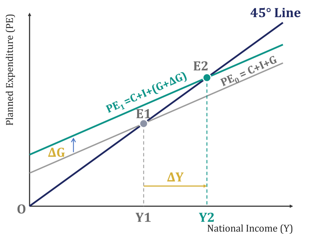
$\Delta PE = \Delta G, \qquad \Delta Y = \frac{\Delta G}{1-c} = k \times \Delta G$

A rise in government spending shifts PE upward by ΔG. Equilibrium moves from E₁ to E₂, and ΔY exceeds ΔG — the multiplier at work.

A change in taxes works indirectly, through consumption. A change $\Delta T$ changes disposable income by $-\Delta T$ , and consumption changes by $c$ times that:

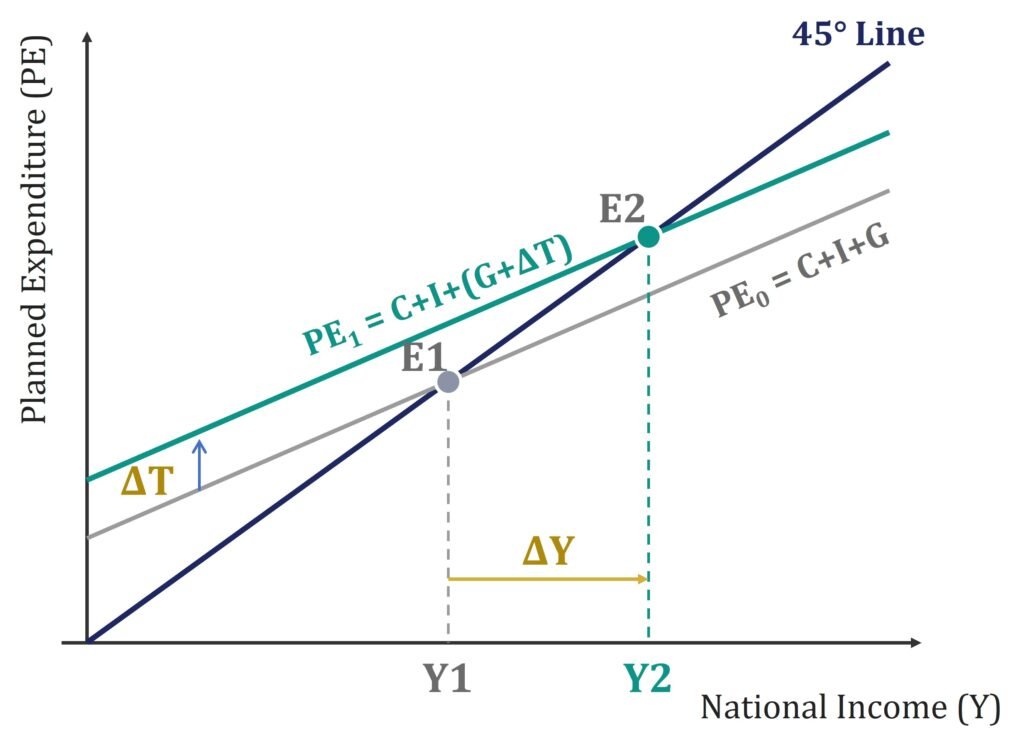
$\Delta PE = -c\,\Delta T, \qquad \Delta Y = \frac{-c\,\Delta T}{1-c}$

A fall in taxes shifts PE upward by MPC × ΔT. Equilibrium moves from E₁ to E₂, and disposable income rises by ΔT and consumption increases by MPC × ΔT.

Notice the tax multiplier, $-c/(1-c)$ , is smaller in absolute size than the spending multiplier, $1/(1-c)$ . A change in $G$ is an immediate, one-for-one injection into spending; a change in $T$ only affects spending indirectly, through the fraction $c$ of it that households choose to consume rather than save.

Worked Example 2 — Fiscal Expansion and the Multiplier at Work

Continue from Example 1, where $Y^{*} = 2{,}200$ with $C_0=200$ , $c=0.8$ , $T_0=200$ , $I_0=150$ , and $G_0=250$ (all PKR billion). Suppose the government raises spending by 50, so $G_1 = 300$ , with everything else unchanged.

Step 1 — New planned expenditure.

$PE_1 = (40 + 0.8Y) + 150 + 300 = 490 + 0.8Y$

Step 2 — New equilibrium.

$Y = 490 + 0.8Y \;\Rightarrow\; 0.2Y = 490$

$Y^{**} = 2{,}450 \text{ (PKR billion)}$

Step 3 — Check against the multiplier.

$\Delta Y = 2{,}450 - 2{,}200 = 250$

$k \times \Delta G = 5 \times 50 = 250 \;\checkmark$

A spending increase of just 50 (PKR billion) raised equilibrium income by 250 — five times as much. This is the multiplier effect in action: the PE line shifted up by exactly 50 at every level of income, and the new intersection with the 45° line landed considerably further to the right.

Key Takeaways

Identity: In a three-sector economy, $Y \equiv C + I + G \equiv AE$ — actual expenditure always equals national income, by definition.
Planned vs. actual: Planned expenditure is intended spending; it equals $Y$ only when the economy is at equilibrium.
Equilibrium: $Y^{*}$ occurs exactly where the PE line crosses the 45° line.
Adjustment: Unplanned inventory changes are the mechanism that pushes output toward equilibrium from either side.
Fiscal policy: A rise in $G$ or a cut in $T$ shifts PE upward and raises equilibrium income by a multiple of the initial change.

The Keynesian Cross is deliberately simple — fixed prices, autonomous investment, no foreign sector — but that simplicity is exactly what makes the core insight so clear: in the short run, spending decisions, not productive capacity, determine where output settles. Once the interest rate is allowed back into the picture, this same cross becomes the IS curve, and the story continues from there.

Share this article

About the author

Muhammad Minhaj Akhtar

Muhammad Minhaj Akhtar is a Lecturer in Economics at Government Graduate College Jauharabad, Pakistan. He holds an M.Phil. in Economics from Quaid-i-Azam University, Islamabad, and an MSc in Economics from the University of Sargodha, where he earned a Silver Medal. His academic passion lies in Econometrics, with a strong focus on applying empirical methods to real-world economic issues. Through MinhajMetrixHub, he shares learning resources, research guidance, and practical econometric insights for students and researchers.