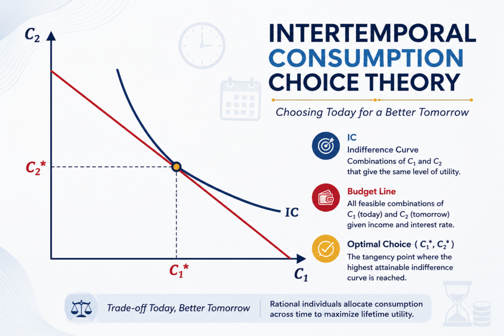
Intertemporal Consumption Choice: Fisher's Model of Consumption and Saving

Intertemporal Consumption Choice: Fisher’s Model of Consumption and Saving

Intertemporal Consumption Choice

Fisher’s Model of Consumption and Saving

Suppose you receive a bonus today. Do you spend all of it now, or do you save part of it for later? Simple income-based theories cannot really answer this question, because they look only at today’s income.

In 1930, the neoclassical economist Irving Fisher offered a different way of thinking about this problem in his book The Theory of Interest. He argued that people do not just think about today. They think about today and tomorrow together, and they choose a spending plan that balances the two. This idea is known as ‘intertemporal consumption choice’, which forms the basis of the Permanent Income Hypothesis in 1957 and the Life Cycle Hypothesis in 1963.

Mainstream Theory of Consumer Behaviour

Mainstream consumer theory assumes that people are rational and try to attain the maximum satisfaction, or utility, out of their income. This satisfaction is limited by a budget constraint — a person can only buy what their income allows.

Classical theory usually looks at this choice within a single time period. It is the same idea used to build ordinary demand curves. Intertemporal choice takes this same logic but considers the future time period also. Instead of asking, “How much of good A versus good B should I buy today?”, it asks, “How much should I consume today versus in the future?”

Key Idea: Intertemporal choice is the decision a person faces when dividing their income between consumption today and consumption at some point in the future.

The Intertemporal Consumption Function

The intertemporal consumption function describes how a person splits their income between present and future consumption, in order to get the highest possible satisfaction over their whole life, given a combined budget limit covering both time periods.

This way of maximising satisfaction across time is also the basic tool used to build broader, economy-wide consumption functions. Irving Fisher was the first to lay out this approach formally, in his 1930 book The Theory of Interest.

Why Look Beyond Today? Keynes vs. Fisher

Keynes’s Absolute Income Hypothesis assumes that current consumption depends only on current income. In this view, the future does not matter for today’s spending decision. But this assumption does not always match how people actually behave.

Fisher’s insight was different. He noticed that, in real life, people weigh present and future consumption together. Spending more today and saving less means having less to spend tomorrow. This is a real trade-off. Fisher’s model captures this by describing rational, forward-looking consumers who plan their consumption across time, rather than one period at a time.

Assumptions of Fisher’s Model

Fisher’s model rests on three key assumptions:

A forward-looking consumer: the consumer plans consumption to get the highest satisfaction over their whole life, not just satisfaction in the present period.
A single intertemporal budget constraint: the consumer’s choices in both periods are limited by one combined budget, covering both periods together.
Two time periods: the consumer lives for two periods only — period 1, called youth, and period 2, called old age.

Three ingredients of the Model

Fisher’s model is built to show three ingredients at once:

Budget constraints: the limits a consumer faces when spreading resources across time.
Preferences: how the consumer feels about consuming now compared to consuming later.
Joint determination: how constraints and preferences work together to decide the best possible level of consumption and saving.

Setting Up the Model: The Intertemporal Budget Constraint

To keep the model simple, Fisher assumes the consumer lives for only two periods:

Period 1 (Youth): the consumer earns income $Y_1$ and consumes $C_1$ .
Period 2 (Old Age): the consumer earns income $Y_2$ and consumes $C_2$ .

The intertemporal budget constraint measures the total resources available for spending across both of these periods.

Step-by-Step Derivation of the Budget Constraint

Step 1: The Budget Constraint in Period 1

In period 1, income $Y_1$ is either consumed as $C_1$ or saved as $S$ :

$Y_1 = C_1 + S$

If $S > 0$ , the consumer is saving part of their income. If $S < 0$ , the consumer is borrowing against income they expect to earn in the future. Rearranging this equation for saving gives:

$S = Y_1 - C_1$

Step 2: The Budget Constraint in Period 2

Saving from period 1 earns a real interest rate, $r$ . In period 2, consumption equals the saved amount plus the interest earned on it, plus the income earned in period 2. Since there is no third period, the consumer spends everything in period 2 and saves nothing further:

$C_2 = Y_2 + (1+r)S$

Worked Example: Suppose the interest rate is $r = 10\%$ , and the consumer saves $S = \text{Rs. } 1{,}000$ in period 1. Then the interest earned is $\text{Rs. } 100$ , giving the consumer an extra Rs. 100 of consumption to enjoy in period 2.

Step 3: Substituting Saving Into the Equation

Now substitute $S = Y_1 - C_1$ , from period 1, into the period-2 equation:

$C_2 = Y_2 + (1+r)(Y_1 - C_1)$

Expanding the bracket gives:

$C_2 = Y_2 + (1+r)Y_1 - (1+r)C_1$

This single equation now links consumption in both periods, $C_1$ and $C_2$ , to income earned in both periods. Rearranging so that consumption terms sit on one side and income terms sit on the other gives:

$(1+r)C_1 + C_2 = (1+r)Y_1 + Y_2$

Step 4: The Intertemporal Budget Constraint (IBC)

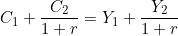
Dividing both sides by $(1+r)$ gives the standard form of the intertemporal budget constraint:

$C_1 + \frac{C_2}{1+r} = Y_1 + \frac{Y_2}{1+r}$

In simple words: the present value of lifetime consumption equals the present value of lifetime income.

Interpreting the Budget Constraint

Special Case: When $r = 0$

If the interest rate is zero, the constraint simplifies to:

$C_1 + C_2 = Y_1 + Y_2$

Here, total consumption across both periods simply equals total income across both periods. No discounting is needed, because saving does not earn any extra return.

General Case: When $r > 0$

When the interest rate is positive, both future consumption and future income are discounted by the factor $\dfrac{1}{1+r}$ . This discount factor measures how much period-1 consumption must be given up in order to gain one extra unit of consumption in period 2.

Deriving the Slope of the Budget Line

Starting from the rearranged constraint:

$(1+r)C_1 + C_2 = (1+r)Y_1 + Y_2$

We can solve this explicitly for $C_2$ :

$C_2 = \big[(1+r)Y_1 + Y_2\big] - (1+r)C_1$

Comparing this to the standard straight-line form, $y = mx + c$ , we can identify the intercept and the slope:

$\text{intercept} = (1+r)Y_1 + Y_2, \qquad \text{slope} = -(1+r)$

So the slope of the intertemporal budget line is:

$\text{Slope} = -(1+r)$

Graphical Presentation of the Budget Line

When plotted with $C_1$ on the horizontal axis and $C_2$ on the vertical axis, the budget line runs from point $M$ to point $P$ , passing through a middle point $N$ :

Figure 1: Intertemporal Budget Line

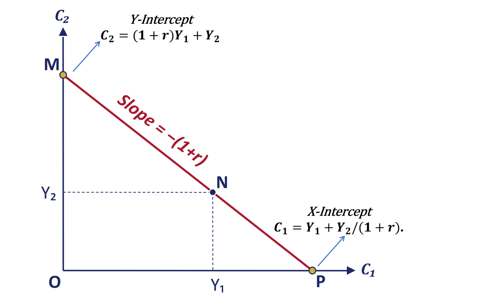
At point M: the consumer saves all of their current income, so $C_1 = 0$ .
At point P: the consumer consumes all of their current income and saves nothing, so $C_2 = 0$ .
Between M and N: the consumer spends less than their income and saves the rest.
Between N and P: the consumer spends more than their income and borrows the difference.
Point N is called the endowment point, where $C_1 = Y_1$ and $C_2 = Y_2$ — that is, the consumer simply consumes their income in each period, without saving or borrowing.

The slope of the full line, from M through N to P, is $-(1+r)$ , exactly as derived above.

Consumer Preferences: Time Indifference Curves

A time indifference curve shows all the combinations of $C_1$ and $C_2$ that give the consumer the same level of satisfaction. Along a single curve, labelled $IC_1$ , points such as $E$ , $F$ , and $G$ all represent equal satisfaction to the consumer.

Figure 2: Time Indifference Curves

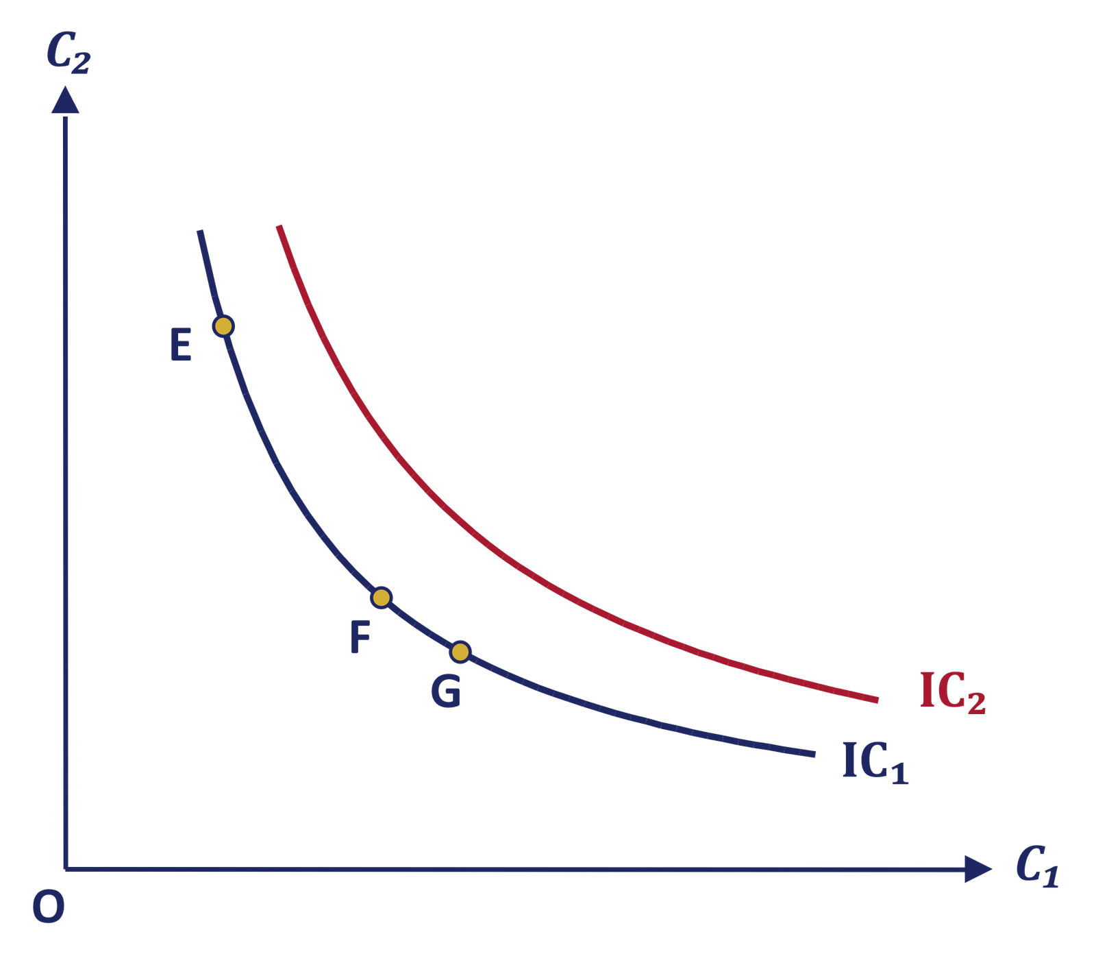
Moving from point $G$ to point $F$ along the curve, $C_1$ falls. To keep satisfaction unchanged, $C_2$ must rise to make up for it. The slope of this curve is called the marginal rate of substitution, or MRS — it tells us how much $C_2$ a consumer is willing to give up for one extra unit of $C_1$ , while keeping satisfaction the same.

A second curve, $IC_2$ , lying above $IC_1$ , represents a higher level of satisfaction. Every point on $IC_2$ is preferred to every point on $IC_1$ .

Optimal Consumption Level

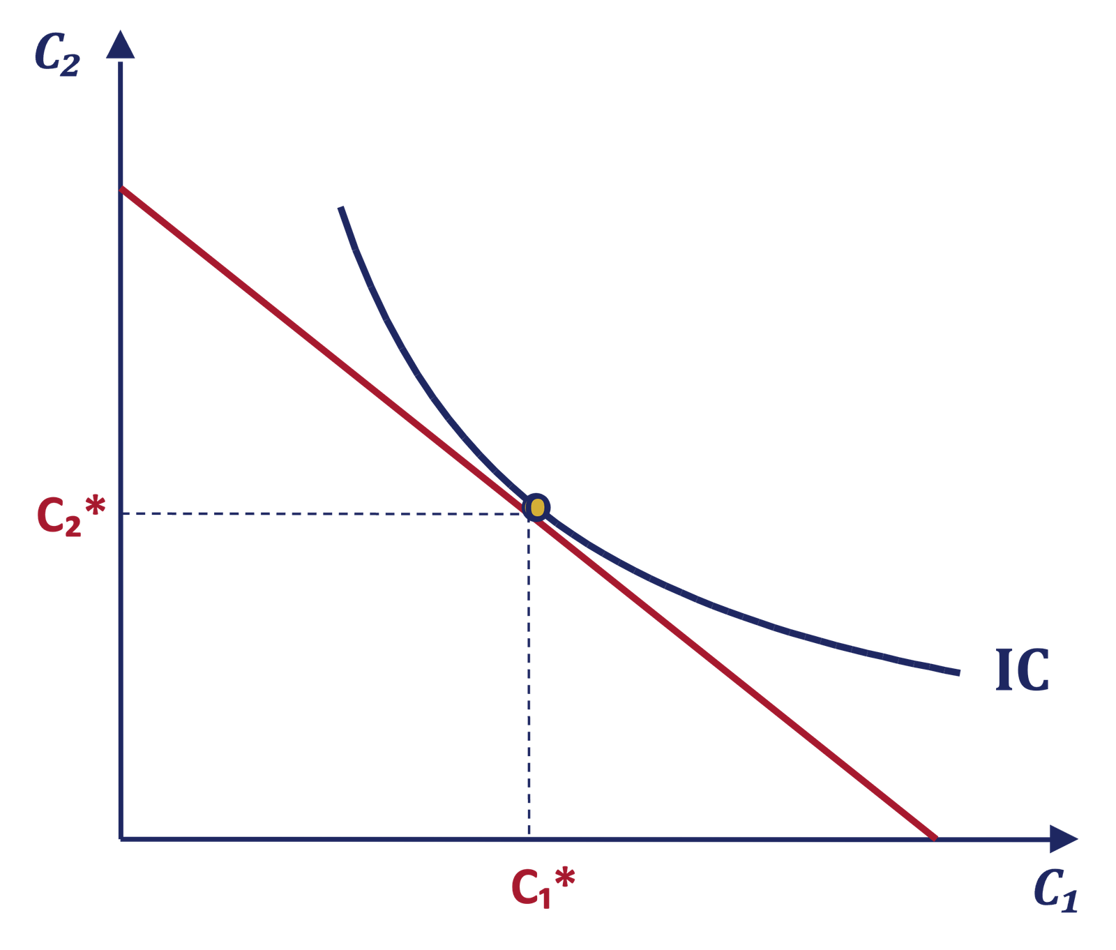
The consumer’s best possible choice, or optimum, occurs where the budget line just touches, or is tangent to, the highest indifference curve the consumer can reach. At this point of tangency, the slope of the budget line equals the slope of the indifference curve:

Figure 3: Optimal Consumption Level

: $(1+r) = MRS$

This tangency condition determines the consumer’s optimal choices, $C_1^{*}$ and $C_2^{*}$ , shown as point $O$ on the standard diagram. At this point, the consumer’s own trade-off between present and future consumption exactly matches the market’s trade-off, which is set by the interest rate.

Key Takeaways: Fisher’s Model in Five Points

Consumers are forward-looking. Their consumption choices weigh both present and future needs together, not just the present.
The intertemporal budget constraint is written as $C_1 + \dfrac{C_2}{1+r} = Y_1 + \dfrac{Y_2}{1+r}$ .
The slope of the budget line is $-(1+r)$ . This represents the price of period-2 consumption, measured in terms of period-1 consumption.
Consumer preferences across time are shown using convex time indifference curves.
The optimal choice occurs where the budget line is tangent to the highest reachable indifference curve, so that $(1+r) = MRS$ .

Conclusion

Fisher’s model of intertemporal consumption choice moved economic thinking beyond the single-period view offered by Keynes. By treating the consumer as a forward-looking planner, balancing present spending against future needs through a single combined budget constraint, Fisher gave economists a clear and flexible framework for studying saving and borrowing decisions. His model remains a foundation for later theories, including the Life Cycle Hypothesis and the Permanent Income Hypothesis, both of which build directly on the idea that consumption choices are made across time, not just within it.

This lecture note is part of an ongoing intermediate macroeconomics series on Minhaj Metrix Hub, covering the development of consumption theory, including Irving Fisher’s model of intertemporal consumption choice.

Suggestions for further readings

The Intertemporal Budget Constraint | EconGraphs

About the author

Muhammad Minhaj Akhtar

Muhammad Minhaj Akhtar is a Lecturer in Economics at Government Graduate College Jauharabad, Pakistan. He holds an M.Phil. in Economics from Quaid-i-Azam University, Islamabad, and an MSc in Economics from the University of Sargodha, where he earned a Silver Medal. His academic passion lies in Econometrics, with a strong focus on applying empirical methods to real-world economic issues. Through MinhajMetrixHub, he shares learning resources, research guidance, and practical econometric insights for students and researchers.