Heteroscedasticity in Econometrics: Meaning, Causes, Tests, and Remedies Explained

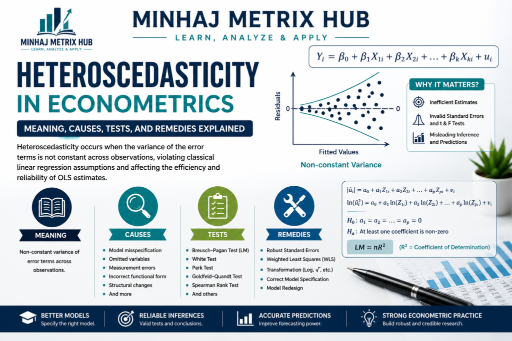
Heteroscedasticity in Econometrics:

Meaning, Causes, Tests, and Remedies Explained

One of the core assumptions of the Classical Linear Regression Model (CLRM) is that the error term has constant variance across all observations. In practice, this assumption is frequently violated, especially when working with cross-sectional data such as household surveys, firm-level data, or cross-country comparisons.

When this assumption breaks down, we enter the world of heteroscedasticity, one of the most important diagnostic issues every BS and MPhil Economics student must understand before interpreting any regression output. This article explains the concept from the ground up, walks through real examples, and covers how to detect and correct it.

Homoscedasticity vs. Heteroscedasticity

Understanding the Core Concept

What is Homoscedasticity?

The term “homo” means equal or same, and “skedasticity” means spread or variance. Homoscedasticity therefore means equal variance. In econometrics, homoscedasticity means that the variance of the error term, conditional on the values of the independent variable X, remains constant across all observations. This is written formally as:

$\operatorname{Var}(u_i \mid X_i)=\sigma^2$

When homoscedasticity holds, the spread of the observed values of Y around the estimated regression line stays roughly the same no matter what value X takes.

What is Heteroscedasticity?

Heteroscedasticity is simply the absence of homoscedasticity. It means the variance of the error term, conditional on X, is not constant. This is written as:

$\operatorname{Var}(u_i \mid X_i)=\sigma_i^2$

The subscript i attached to $\sigma_i^2$ signals that the variance changes as X changes. Under heteroscedasticity, the spread of Y values around the regression line is not uniform across observations, it may widen, narrow, or follow some other systematic pattern as X increases.

What Does Heteroscedasticity Look Like?

Consider a simple two-variable regression model:

$Y_i=\beta_0+\beta_1X_i+u_i$

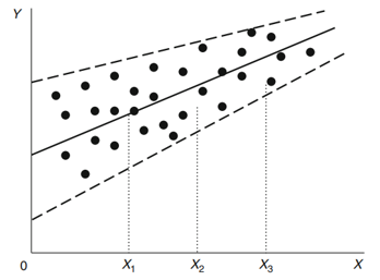
If we plot the scatter of Y against X along with the fitted regression line, three broad patterns can emerge:

Figure 1: Data with equal spread

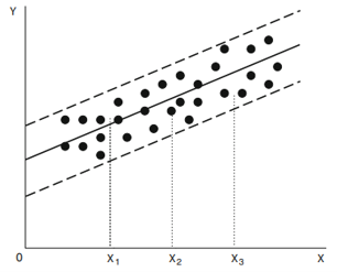
Figure 2: Data with increasing spread

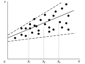
Figure 3: Data with decreasing spread

Equal spread across all values of X: Points cluster closely and evenly around the regression line regardless of whether X is small or large. This is the homoscedastic case (Figure 1).
Increasing spread as X increases: Y values fan outward from the regression line as X grows larger, so higher values of X are associated with greater variability in Y. This is one common form of heteroscedasticity (Figure 2).
Decreasing spread as X increases: The spread around the regression line is wide at low values of X and narrows as X increases. This is the opposite pattern of heteroscedasticity (Figure 3).

Both the increasing-spread and decreasing-spread patterns indicate that the error variance is not constant.

Real-World Examples of Heteroscedasticity

Example 1: Household Income and Consumption

A classic example of the increasing-spread pattern comes from income and consumption behavior, which applies directly to household data collected in Pakistan through surveys like HIES or PSLM.

Economic theory tells us that consumption rises with income, but at low income levels, households have very little flexibility, since a large share of a low-income household’s budget in Pakistan is committed to food, rent, and transport, leaving little room for variation. As a result, consumption patterns among low-income households look fairly similar, so the spread is small.

Higher-income households, however, have far more discretion: some save heavily, some invest in property or the stock market, and some spend lavishly. This greater freedom of choice produces a much wider spread in consumption among richer households than among poorer ones, a textbook case of heteroscedasticity.

Example 2: Data Collection Quality and Error-Learning

The opposite pattern, decreasing spread, can be illustrated through improvements in data collection or through error-learning behaviour. For instance, large commercial banks in Pakistan with sophisticated data-processing systems can estimate customer credit risk with fewer errors than smaller banks relying on manual processes, so variability in their estimates is lower.

Similarly, in an error-learning model, if Y represents a student’s test score and X represents the number of times the student has attempted a similar test or hours spent preparing, we would expect the variability in scores to shrink as X (practice or preparation) increases, since experience reduces the chance of large errors.

Example 3: Manufacturing Output and GDP Across Economies

A further illustration involves comparing manufacturing sector output (Y) against GDP (X) across a group of countries. In cross-country data, two patterns typically emerge together: economies with larger GDP tend to have larger manufacturing output, and more importantly for our purposes, larger economies also show much greater variation in manufacturing output relative to their size than smaller economies do.

Because bigger economies pursue very different industrial strategies (some are manufacturing-heavy, others services-heavy), the variability among them is naturally larger, again reflecting heteroscedasticity in cross-sectional comparisons.

Consequences of Heteroscedasticity

OLS estimators remain linear, unbiased, and consistent even under heteroscedasticity.
However, they are no longer minimum variance, meaning they lose efficiency and are no longer BLUE (Best Linear Unbiased Estimators).
The variances and standard errors of the OLS estimates become biased because the usual estimator of $\sigma^2$ which assumes constant variance, is no longer an unbiased estimator of the true $\sigma^2$ .
As a result, the standard confidence intervals and hypothesis tests based on the t-distribution and F-distribution become unreliable.
Standard errors are often underestimated, which inflates t-statistics and F-statistics beyond their true values.
This inflation leads researchers to reject the null hypothesis more often than they should, creating a false impression of statistical significance.

Sources and Causes of Heteroscedasticity

Several factors commonly give rise to heteroscedasticity in applied econometric work:

Consumption patterns: As explained above, low-income households show little variability in spending while high-income households show much more, causing the error variance to rise with income.
Error-learning models: As economic agents gain experience, the likelihood of making large errors decreases, reducing the error variance over time or across observations.
Data collection techniques: Improvements in how data is gathered and processed tend to reduce measurement-related error variance.
Outliers: Observations that are unusually large or small relative to the rest of the sample can cause the error variance to differ systematically.
Specification bias: This occurs when a model is incorrectly specified — for example, using a linear demand function when a log-linear form is more appropriate, or omitting a relevant variable such as the price of substitute goods from a demand equation.
Skewness in regressors: If one or more explanatory variables are skewed rather than symmetrically distributed, this can generate heteroscedasticity in the error term.
Cross-sectional data: Heteroscedasticity is especially common in cross-sectional data covering individuals, households, firms, or provinces, since these units often differ substantially in size and scale.
Measurement errors: Errors in measuring an independent variable can introduce heteroscedasticity — for example, higher-income respondents in a Pakistani household survey may under-report or misreport their income with less precision than lower-income respondents, causing the error variance to grow with income.

How to Detect Heteroscedasticity

Informal Method: Graphical Inspection

In a two-variable model, a simple scatterplot of Y against X can reveal heteroscedasticity if the spread of points around the regression line visibly widens or narrows as X changes.

In a multiple regression model with more than one explanatory variable, heteroscedasticity is typically detected by plotting the squared residuals against either the fitted (estimated) values of the dependent variable or against individual explanatory variables.

A residual plot that widens, narrows, or displays a noticeable pattern indicates heteroscedasticity. In contrast, when the residuals are randomly scattered around zero with a roughly constant spread, the data exhibit homoscedasticity.

Formal Statistical Test

The Goldfeld-Quandt Test

The Goldfeld-Quandt test, developed in 1965, is the most widely used formal test for heteroscedasticity in simple regression models. It rests on the idea that if the error variance is genuinely constant across the sample, the variance estimated from one part of the sample should match the variance estimated from another part. This test requires prior knowledge of which variable is most likely related to the variance of the error term. The procedure is as follows:

Step 1: Arrange the observations of the suspected X variable in descending order (from highest to lowest), and rearrange the corresponding Y values accordingly.

Step 2: Split the ordered data into two subsamples, omitting a middle block of c observations, where c is typically chosen between one-sixth and one-third of the total sample size. Each of the two remaining subsamples will then contain $\frac{1}{2}(n-c)$ observations.

Step 3: Run separate OLS regressions on each subsample and obtain the residual sum of squares from each, RSS₁ and RSS₂.

Step 4: Compute the F-statistic:

$F=\frac{RSS_1}{RSS_2}$

This statistic follows an F-distribution with degrees of freedom:

$F_{\text{crit}}=\left[F_{\alpha/2}(n-c-k),\;F_{1-\alpha/2}(n-c-k)\right]$

Step 5: State the hypotheses tested:

$H_0:\sigma_1^2=\sigma_2^2,\qquad H_1:\sigma_1^2\neq\sigma_2^2$

Step 6: If the calculated F-statistic exceeds the critical F-value, we reject the null hypothesis and conclude that the error variances of the two subsamples differ significantly, confirming the presence of heteroscedasticity.

Spearman’s Rank Correlation Test

This test checks whether the absolute residuals from a regression are correlated with the explanatory variable; if they are, this signals that the error variance changes systematically with X.

A Numerical Example

Y	X
12.4	12.1
14.4	21.4
14.6	18.7
16	21.7
11.3	12.5
10	10.4
16.2	20.8
10.4	10.2
13.1	16
11.3	12

Step 1: State the hypotheses.

$H_0:\ \text{Variance of the error term is constant (homoscedasticity)}$

$H_a:\ \text{Variance of the error term is not constant (heteroscedasticity)}$

Step 2: Fit the regression and obtain residuals. Using a sample of 10 observations on Y and X, suppose OLS gives the fitted line:

$\hat{Y}_i = 5.8194 + 0.459X_i$

Step 3: Compute the absolute residuals $|\hat{u}_i|$ for each observation, then rank both the absolute residuals and the X values (in either ascending or descending order), and calculate the difference in ranks, d, and its square, $d^2$ , for each observation. Summing across all 10 observations in this worked example gives:

$\sum d_i^2 = 110$

The Spearman’s rank correlation coefficient is calculated as:

$r_s = 1 - \frac{6\sum d_i^2}{n(n^2-1)}$

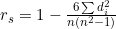
Substituting the values:

$r_s = 1 - \frac{6 \times 110}{10(10^2-1)}$

$r_s = 1 - \frac{660}{990} = 1 - 0.6667 = 0.3333$

Step 4: Test the significance of $r_s$ , using a t-test, assuming the population rank correlation is zero and n is greater than 8:

$t=\frac{r_s\sqrt{n-2}}{\sqrt{1-r_s^2}}$

$t=\frac{0.3333\sqrt{8}}{\sqrt{1-(0.3333)^2}}$

$t=\frac{0.3333\times 2.8284}{\sqrt{0.8889}}$

$t=\frac{0.9428}{0.9428}\approx 1.00$

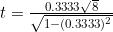
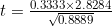
Step 5: Compare the computed t-value to the critical t-value from the t-table. Since the computed t-value of approximately 1.00 is well below any conventional critical value, we fail to reject the null hypothesis and conclude that there is no significant evidence of heteroscedasticity in this particular sample.

The Park Test

The Park test extends the idea of relating residual variance to an explanatory variable using a log-linear specification.

Step 1: Run the original regression:

$Y_i=\beta_0+\beta_1X_{1i}+\beta_2X_{2i}+\cdots+\beta_kX_{ki}+u_i$

Step 2: Obtain the residuals $\hat{u}_i$ .

Step 3: Run an auxiliary regression of the log of the squared residuals on the logs of the explanatory variables:

$\ln(\hat{u}_i^{\,2})=a_0+a_1\ln(Z_{1i})+a_2\ln(Z_{2i})+\cdots+a_p\ln(Z_{pi})+v_i$

Step 4: State the null and alternative hypotheses of homoscedasticity:

$H_0:\ a_1=a_2=\cdots=a_p=0$

$H_a:$ at least one coefficient is non-zero

The alternative hypothesis means that the variable affects the residual variance.

Step 5: Compute the LM statistic as $LM=nR^2$ , where $R^2$ is the coefficient of determination from the auxiliary regression.

Step 6: Conclusion, If the LM statistic exceeds the critical chi-square value (or equivalently, if the p-value is below the chosen significance level, commonly 0.05), reject the null hypothesis and conclude that heteroscedasticity is present.

The Glejser Test

The Glejser test follows the same logic as the Park test but uses the absolute value of the residuals rather than their log-squared values in the auxiliary regression:

$|\hat{u}_i|=a_0+a_1(Z_{1i})+a_2(Z_{2i})+\cdots+a_p(Z_{pi})+v_i$

The hypotheses, $LM=nR^2$ statistic, and the decision rule are identical in structure to the Park test: reject the null hypothesis of homoscedasticity if the LM statistic exceeds its critical value or if the associated p-value falls below the significance level.

Other Common Tests

Beyond the tests detailed above, several other formal tests are widely used in applied econometrics to detect heteroscedasticity, including the Breusch-Pagan LM test and White’s test. Both are commonly available as built-in post-estimation commands in Stata and EViews, making them convenient choices for students working with real datasets.

How to Resolve Heteroscedasticity

Weighted Least Squares (WLS)

Weighted Least Squares (WLS) is a regression technique specifically designed to correct heteroscedasticity. Unlike OLS, which treats every observation equally, WLS assigns a weight to each observation based on the inverse of its estimated error variance:

$w_i=\frac{1}{\sigma_i^2}$

Observations with lower error variance, meaning they lie closer to the true regression relationship and carry more reliable information, receive higher weights, while observations with higher error variance receive lower weights.

By minimizing a weighted sum of squared residuals rather than a simple, equally-weighted sum, WLS restores efficiency to the parameter estimates and produces valid standard errors, giving BLUE estimates even in the presence of heteroscedasticity. Estimators obtained this way are called WLS estimators.

Generalized Least Squares (GLS)

Generalized Least Squares (GLS) is a more general technique used whenever the OLS assumptions of homoscedasticity and no autocorrelation are violated. GLS works by transforming the original variables so that the transformed variables satisfy the classical regression assumptions and then applying OLS to these transformed variables.

The resulting GLS estimators are BLUE, even when the original data suffered from heteroscedasticity, autocorrelation, or both.

WLS vs. GLS: Key Differences

Error structure: WLS assumes errors are independent but not identically distributed, meaning variances differ across observations but are uncorrelated with each other. GLS can handle both unequal variances and correlated errors (autocorrelation) simultaneously.

Weighting: In WLS, weights are simply the inverse of each observation’s error variance, and the resulting weight matrix is diagonal. In GLS, the weight matrix can be non-diagonal, capturing both variances and covariances between observations.

Special case relationship: WLS is technically a special case of GLS that applies when the errors are uncorrelated with one another, so the weight matrix reduces to a diagonal form.

Use case: Choose WLS when only heteroscedasticity is present. Choose GLS when both heteroscedasticity and autocorrelation need to be corrected simultaneously.

Other Remedial Measures

Beyond WLS and GLS, several practical remedies are commonly applied in econometric practice:

Use robust standard errors, which remain valid for hypothesis testing even in the presence of heteroscedasticity, without needing to change the estimation method itself.
Apply a log transformation to the dependent or independent variables, which often compresses the scale of the data and reduces both variability and the influence of outliers.
Convert the original dependent variable into per-capita or growth-rate form, which is a particularly common fix in macroeconomic and cross-country studies where scale differences between countries or regions drive heteroscedasticity.
Use Weighted Least Squares, which downweights observations coming from segments of the data with higher error variance.
Use Generalized Least Squares, which can simultaneously correct both heteroscedasticity and autocorrelation.
Add omitted variables that were causing model misspecification, since specification bias is itself a common source of heteroscedasticity.

Conclusion

Heteroscedasticity is one of the most common violations of the classical regression assumptions, particularly in cross-sectional economic data such as household surveys, firm-level datasets, and cross-country comparisons frequently used in economic research.

While it does not bias OLS coefficient estimates, it undermines their efficiency and renders standard hypothesis tests unreliable. Weighted Least Squares, or Generalized Least Squares, allow researchers to restore the reliability of their estimates and proceed with confidence.

Suggestions for further readings

Multicollinearity: Types, Concequences, Causes, Detection & Remedies

About the author

Muhammad Minhaj Akhtar

Muhammad Minhaj Akhtar is a Lecturer in Economics at Government Graduate College Jauharabad, Pakistan. He holds an M.Phil. in Economics from Quaid-i-Azam University, Islamabad, and an MSc in Economics from the University of Sargodha, where he earned a Silver Medal. His academic passion lies in Econometrics, with a strong focus on applying empirical methods to real-world economic issues. Through MinhajMetrixHub, he shares learning resources, research guidance, and practical econometric insights for students and researchers.