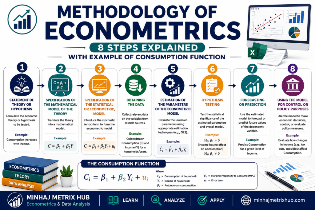
Methodology of Econometrics: 8 Steps Explained with an Example

Every empirical study in economics, whether it involves estimating inflation dynamics or testing the consumption behaviour of households in a particular country, follows a disciplined research path before any regression output can be trusted. This path is called econometric methodology. While several schools of thought exist on how econometric research should proceed, the traditional or classical methodology remains the most widely taught and applied framework, especially at the undergraduate and graduate levels. This article walks through all eight steps of this methodology using a single running example: estimating the consumption function of households in Punjab, Pakistan, so you can see how each step connects to the next in a real applied setting.

Step 1: Statement of Theory or Hypothesis

The starting point of any econometric study is a testable statement derived from economic theory. According to Keynes’s Absolute Income Hypothesis, as disposable income rises, households increase their consumption expenditure, but by a smaller amount than the rise in income itself. In other words, the Marginal Propensity to Consume (MPC) lies between 0 and 1. This means that as a household earns more disposable income per month, its spending on food, utilities, and other necessities will rise, but not in the same proportion as income, since part of the additional income is saved.

This step gives us our working hypothesis: there is a positive relationship between household consumption expenditure (CONS) and disposable income (INC), with the MPC strictly between 0 and 1.

Step 2: Specification of the Mathematical Model

Once the hypothesis is stated, it must be translated into a precise mathematical equation. The functional form can be chosen either by plotting a scatter diagram of the data or by relying on economic theory itself. For a simple Keynesian consumption function, a linear form is typically used:

$CONS = \beta_0 + \beta_1 INC$

subject to the theoretical restriction

$0 < \beta_1 < 1$

Here, CONS is the dependent variable, representing monthly household consumption expenditure in Pakistani Rupees, and INC is the independent variable, representing monthly disposable household income in Pakistani Rupees. The parameter is the intercept, interpreted in economic terms as autonomous consumption, the amount a household would spend even with zero income, financed through savings or borrowing. The parameter is the slope and represents the MPC, the effect of a one-unit change in income on consumption.

Step 3: Specification of the Econometric Model

A mathematical model is deterministic; it assumes an exact relationship with no deviation. Real household survey data from Pakistan, such as that collected through the Household Integrated Economic Survey (HIES) or the Pakistan Social and Living Standards Measurement (PSLM) survey, never fit a straight line perfectly. Two households with identical income levels will rarely report identical consumption, because factors like family size, remittances from abroad, health shocks, or local prices also matter. To account for this, a stochastic error term (u) is added, converting the mathematical model into an econometric model:

$CONS = \beta_0 + \beta_1 INC + u$

The error term u absorbs the effect of all the omitted variables, measurement errors, and pure randomness that influence consumption but are not explicitly captured by income alone.

Step 4: Obtaining the Data

With the econometric model specified, the next task is to collect actual data to estimate it. In practice, this is the responsibility of an economic statistician or data analyst. For a study on Pakistani household consumption, data could be sourced from the Pakistan Bureau of Statistics (HIES/PSLM datasets), the State Bank of Pakistan, or international repositories such as the World Development Indicators (WDI), International Financial Statistics (IFS), OECD Economic Outlook, Luxembourg Income Study (LIS), and Penn World Table (PWT).

Depending on the research design, the data collected could take several forms:

• Time series data—for example, Pakistan’s aggregate consumption and income figures recorded annually from 2000 to 2024.
• Cross-sectional data — for example, consumption and income figures for 500 households in Punjab surveyed in a single year.
• Pooled data—combining cross-sections from different years without tracking the same households over time.
• Panel data — following the same set of households across multiple years, which is the richest but hardest data type to collect.

For our example, suppose a researcher collects cross-sectional data on monthly consumption and disposable income from 300 households across Punjab.

Step 5: Estimation of the Parameters

Once data is available, the numerical values of and are estimated using an econometric technique, most commonly Ordinary Least Squares (OLS) or, in some cases, Maximum Likelihood Estimation (MLE). Suppose the OLS regression on our 300-household sample from Punjab produces the following estimated consumption function, with figures in Pakistani Rupees:

$\widehat{CONS} = 3200 + 0.74 \, INC$

The hat symbol over CONS indicates that this is the estimated, or fitted, value of consumption rather than the actual observed value. Here, the estimated autonomous consumption is Rs. 3,200 per month, and the estimated MPC is 0.74, meaning that for every additional Rs. 100 of disposable income, a household in the sample increases its consumption by roughly Rs. 74.

Step 6: Hypothesis Testing

An estimated coefficient is only useful if it is statistically reliable rather than a product of chance. This step tests whether the estimated slope truly reflects the population relationship or could plausibly be zero. The hypotheses are formally stated as:

$H_0: \beta_1 = 0$

$H_a: \beta_1 \neq 0$

Tools used here include the t-test for individual coefficients, the F-test for overall model significance, and, in more advanced settings, the Chi-square test or ANOVA. If the p-value associated with is less than the chosen significance level (commonly 0.05), the null hypothesis is rejected, and we conclude that disposable income does have a statistically significant effect on household consumption in Punjab, with an estimated MPC of 0.74.

Step 7: Forecasting or Prediction

Once the model passes hypothesis testing and is not rejected, it can be used to forecast future or out-of-sample values. Suppose a household in Punjab reports a monthly disposable income of Rs. 60,000. Using the estimated model:

$\widehat{CONS} = 3200 + 0.74 \times 60000 = 47{,}600$

The model predicts this household will spend approximately Rs. 47,600 per month on consumption. If the household’s actual reported consumption was Rs. 46,500, the forecast error would be Rs. 1,100, meaning the model slightly overestimated actual spending. Such forecast errors are normal; they do not necessarily mean the model is flawed. Forecast accuracy across a full sample is typically evaluated using measures such as Mean Squared Error (MSE), Mean Absolute Error (MAE), and Mean Absolute Percentage Error (MAPE).

Step 8: Using the Model for Control or Policy Purposes

The final step puts the estimated model to practical use in policy analysis. Suppose Pakistan enters a period of slowing economic growth, and the government wants to boost aggregate demand. Since consumption is a major component of aggregate demand, and our model shows that a Rs. 100 rise in disposable income raises consumption by about Rs. 74, the government could use a tax reduction to raise households’ disposable income directly. Given the estimated MPC of 0.74, policymakers can approximate how much additional consumption spending a given tax cut is likely to generate across the economy, informing the design of fiscal stimulus measures.

Conclusion

The eight steps of econometric methodology, from stating a theory to using the estimated model for policy, form a logical chain in which each step depends on the one before it. Using a single example throughout, the Keynesian consumption function for Punjabi households shows how an abstract theoretical claim about the Marginal Propensity to Consume can be transformed step by step into a concrete, testable, and policy-relevant empirical model. For BS Economics students, mastering this sequence is the foundation for every applied econometrics project, thesis, or research paper that follows.

Q/A Section

Q1: What are the main steps of econometric methodology?

A1: Classical econometric methodology follows eight steps: stating the theory or hypothesis, specifying the mathematical model, converting it into a statistical (econometric) model, obtaining data, estimating parameters, testing hypotheses, forecasting, and using the model for policy or control purposes.

Q2: What is the difference between a mathematical model and an econometric model?

A2: A mathematical model expresses a theory as an exact equation with no room for error, while an econometric model adds a stochastic error term to account for randomness, omitted variables, and measurement issues that affect real-world data.

Q3: Why is the error term included in an econometric model?

A3: The error term captures the influence of unobserved factors, omitted variables, and measurement errors that affect the dependent variable but are not explicitly included in the model, making the equation realistic for empirical estimation.

Q4: What data sources are commonly used in econometric research?

A4: Common sources include the World Development Indicators (WDI), International Financial Statistics (IFS), OECD Economic Outlook, Luxembourg Income Study (LIS), and Penn World Table (PWT), along with national sources such as the Pakistan Bureau of Statistics.

Q5: How is an estimated econometric model used for policy purposes?

A5: Once a model is validated through hypothesis testing, policymakers can manipulate control variables — such as taxes or interest rates — to influence the target variable, for example, increasing disposable income to raise aggregate consumption during a recession.