Autocorrelation in Econometrics: Causes, Consequences, Detection, and Remedies

Table of Contents

Autocorrelation in Econometrics

Causes, Consequences, Detection, and Remedies

Much of applied macroeconomic research, from modelling GDP growth to forecasting inflation or exchange rate movements, relies on time series data. However, time series data presents its own set of estimation challenges, and one of the most significant is autocorrelation. This article explains what time series data is, why autocorrelation arises, how to detect it formally using the Durbin-Watson test with a full worked numerical example, and how to correct it.

What is Autocorrelation?

One of the core assumptions of the Classical Linear Regression Model (CLRM) is that successive values of the error term are independent of each other; the disturbance associated with any one observation should not be influenced by the disturbance associated with any other observation. Formally:

$\operatorname{Cov}(u_i,u_j \mid X_i,X_j)=E(u_i u_j)=0,\quad i\neq j$

This condition, where the covariance and correlation between different disturbance terms are all zero, is called serial independence.

When this assumption is violated, that is, when the error term for one observation is correlated with the error term for another observation, the result is called autocorrelation, or serial correlation:

$\operatorname{Cov}(u_i,u_j \mid X_i,X_j)\neq 0,\quad i\neq j$

Autocorrelation is a special case of correlation. Rather than measuring the correlation between two different variables, X and Y, it measures the correlation between successive values of the same variable. In a regression context, this means that autocorrelation occurs when error terms are correlated over time — the error in the current period is influenced by lagged, or past, error terms.

The Autocorrelation Coefficient

The autocorrelation coefficient, denoted by rho ( $\rho$ ), measures the magnitude and strength of serial correlation. It ranges between -1 and +1. For a regression model $Y_t=\beta_0+\beta_1X_t+u_t$ , the first-order autocorrelation between error terms is written as:

$u_t=\rho u_{t-1}+v_t$

and can be calculated as:

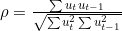
$\rho=\frac{\sum u_tu_{t-1}}{\sqrt{\sum u_t^2\sum u_{t-1}^2}}$

In large samples, this simplifies approximately to:

$\rho=\frac{\sum u_tu_{t-1}}{\sum u_{t-1}^{2}}$

If $\rho$ , there is no autocorrelation between the errors.
If $\rho$ approaches unity (either -1 or +1), it indicates a high degree of autocorrelation.
A value of $\rho=+1$ represents perfect positive autocorrelation, while $\rho=-1$ represents perfect negative autocorrelation.

Patterns of Autocorrelation

When residuals are plotted against time, several distinct patterns can emerge. A cyclical pattern in the residuals is one sign of autocorrelation. An upward or downward linear trend in the disturbances is another. In some cases, both linear and quadratic trend components appear together in the residual pattern. In Figure 1 part a to d show patterns of autocorrelation.

Figure 1: Patterns of Autocorrelation

: Patterns of Autocorrelation

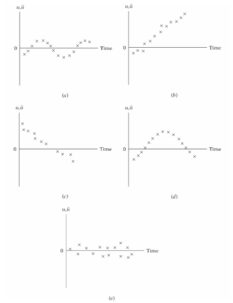
Only when the residuals show no systematic pattern at all, scattering randomly around zero, does the data support the non-autocorrelation assumption of the classical linear regression model. In Figure 1, part e shows no patterns of autocorrelation.

Consequences of Autocorrelation

OLS estimators remain linear, unbiased, and consistent, even in the presence of autocorrelation.
However, they are no longer efficient — they no longer have minimum variance and are therefore no longer BLUE (Best Linear Unbiased Estimators).
The variances and standard errors of the OLS estimators become biased and inconsistent.
As a result, the usual t-tests, F-tests, and confidence intervals become unreliable, leading to misleading statistical inferences.
$R^2$ values and t-statistics tend to become inflated.
Prediction and forecasting based on the model become unreliable.

Causes and Sources of Autocorrelation

Inertia: Macroeconomic time series such as GNP, price indices, output, and employment tend to exhibit inertia, or sluggishness — a resistance to sudden change — which shows up as business cycle behavior and generates autocorrelated errors.
Specification Bias — Omitted Variables: Excluding an important explanatory variable is a key cause of autocorrelation. Its effect gets absorbed into the error term, and if that omitted variable itself carries a trend, the error term becomes correlated over time.
Specification Bias — Incorrect Functional Form: Using the wrong functional form may also lead to autocorrelation. For example, if the true relationship is $MC_{t} = \beta_{0} + \beta_{1}Q_{t} + \beta_{2}Q_{t}^{2} + u_{t}$ but a researcher wrongly estimates $MC_{t} = \beta_{0} + \beta_{1}Q_{t} + u_{t}$ , the omitted $Q_{t}^{2}$ term gets absorbed into the error, so $u_{t} = \beta_{2}Q_{t}^{2} + v_{t}$ . If $Q_{t}$ trends over time, this produces autocorrelation in the error term.
Cobweb Phenomenon: Agricultural supply commonly reflects the cobweb phenomenon, where supply in period t depends on the price of the commodity in the previous period, t-1:

$Supply_{t} = \beta_{0} + \beta_{1} P_{t-1} + u_{t}$

This is highly relevant to Pakistan’s agricultural sector, where farmers’ planting decisions for crops such as wheat or cotton are often influenced by the prices from the previous season.

Lags: Consumption expenditure in period t often depends not only on current income but also on the household’s own consumption in the previous period, t-1, because consumption habits do not change abruptly:

$Consumption_t = \beta_0 + \beta_1 Income_t + \beta_2 Consumption_{t-1} + u_t$

This specification is called autoregression. If the lagged consumption term is omitted from the model, its effect is absorbed into the error term, producing autocorrelation.

Data Manipulations: Changing the frequency of data — for example, converting monthly data into quarterly data — as well as interpolating or extrapolating missing values, can introduce autocorrelation into the error terms.
Data Transformations: Converting raw data into log form or difference form can also introduce autocorrelation.
Nonstationarity: Time series data is frequently nonstationary, exhibiting trends. When nonstationary Y and X variables are used in a regression, the resulting error term also becomes nonstationary, exhibiting its own increasing or decreasing trend and generating autocorrelation.
Measurement Errors: Systematic errors in how a variable is measured over time can likewise generate autocorrelation.

Detecting Autocorrelation

Informal Method: Graphical Inspection

Autocorrelation can be inspected informally by plotting residuals against time or by plotting residuals against their own lagged values. From these plots, several conclusions can be drawn:

If the residuals in successive time periods follow a regular pattern — such as a sawtooth or cyclical shape — this indicates autocorrelation.
If the residuals show no regular pattern, this suggests the absence of autocorrelation.
More specifically, if the residuals do not change sign frequently, so that a run of positive residuals is followed by a run of negative residuals, this points to positive autocorrelation.
If the residuals change sign frequently — a positive residual immediately followed by a negative one, and so on — this points to negative autocorrelation.

Formal Method: The Durbin-Watson Test

The Durbin-Watson test, developed by J. Durbin and G. S. Watson in 1951, is the most widely used test for detecting first-order autocorrelation in time series regressions. It applies even to small samples, though it is only appropriate for testing a First Order Autoregressive Scheme (FOARS).

Assumptions of the Durbin-Watson Test:

The regression model includes an intercept term.

$Y_{t} = \beta_{0} + \beta_{1}X_{t} + u_{t}$

The explanatory variables are non-stochastic, meaning they are fixed in repeated sampling and are not correlated with the error term.
Only first-order autocorrelation is assumed between the error terms.
$u_{t} = \rho u_{t-1} + v_{t}$
The regression model should not include a lagged value of the dependent variable as an explanatory variable. In other words, the model should not take the following form:
$Y_{t} = \beta_{0} + \beta_{1}X_{t} + \beta_{2}Y_{t-1} + u_{t}$
The error term is assumed to be normally distributed.

Procedure of the Durbin-Watson Test:

Step 1: Run the Ordinary Least Squares (OLS) regression and obtain the residuals, $\hat{u}_{t}$ .

Step 2: Compute the Durbin–Watson (DW) statistic.

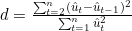
$d=\frac{\sum_{t=2}^{n}(\hat{u}_t-\hat{u}_{t-1})^2}{\sum_{t=1}^{n}\hat{u}_t^2}$

The Durbin–Watson statistic is the ratio of the sum of squared differences between successive residuals to the residual sum of squares (RSS).

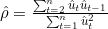
Step 3: For large samples, the Durbin–Watson statistic is approximately related to the estimated first-order autocorrelation coefficient.

$d \approx 2(1-\hat{\rho})$

where

$\hat{\rho}=\frac{\sum_{t=2}^{n}\hat{u}_{t}\hat{u}_{t-1}}{\sum_{t=1}^{n}\hat{u}_{t}^{2}}$

Step 4: For the given sample size ( $n$ ) and the number of explanatory variables ( $k$ ), obtain the critical lower bound ( $d_{L}$ ) and upper bound ( $d_{U}$ ) values from the Durbin–Watson tables and compare them with the calculated Durbin–Watson statistic to conclude the presence or absence of first-order autocorrelation.

Step 5: Apply the following decision rules:

Condition	Conclusion
d < dL	Positive autocorrelation
dL ≤ d ≤ dU	Inconclusive
dU < d < 4 − dU	No autocorrelation
4 − dU ≤ d ≤ 4 − dL	Inconclusive
d > 4 − dL	Negative autocorrelation

As a quick reference, use the following table:

Autocorrelation Coefficient (ρ)	DW Statistic (d)	Conclusion
ρ=0	d = 2	No autocorrelation
ρ>0	d < 2	Positive autocorrelation
ρ<0	d > 2	Negative autocorrelation

Worked Numerical Example of the Durbin-Watson Test

Consider annual time series data on consumption (Y) and disposable income (X) for a country over the period 1957 to 1968. Check for autocorrelation using the Durbin-Watson test.

Year	Consumption (Y)	Income (X)
1957	11378	11617
1958	13012	13297
1959	15263	15790
1960	16873	18017
1961	17764	19314
1962	18857	20198
1963	20074	21512
1964	21439	23124
1965	22833	24724
1966	24205	26175
1967	25307	27219
1968	27020	28915

Step 1: State the hypotheses:

$H_0:\ \rho=0$ (no autocorrelation)

$H_a:\ \rho\neq0$ (autocorrelation, positive or negative))

Step 2: Run the OLS regression on the following model using data and obtain the residuals, $\hat{u}_t$

$Y_t=\beta_0+\beta_1X_t+u_t$

where

$u_t=\rho u_{t-1}+v_t$

Step 3: Compute the d-statistic from the following formula

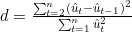
$d=\frac{\sum_{t=2}^{n}\left(\hat{u}_t-\hat{u}_{t-1}\right)^2}{\sum_{t=1}^{n}\hat{u}_t^2}$

Calculation Table

Year	C	Y	$\hat{C}$	$\hat{u}_t$	$\hat{u}_{t-1}$	$\hat{u}_t^2$	$\hat{u}_t-\hat{u}_{t-1}$	$\left(\hat{u}_t-\hat{u}_{t-1}\right)^2$
1957	11378	11617	11314.31	63.68664		4055.988
1958	13012	13297	12808.15	203.8547	63.68664	41556.73	140.1681	19647.08
1959	15263	15790	15024.89	238.1148	203.8547	56698.65	34.26009	1173.754
1960	16873	18017	17005.1	-132.102	238.1148	17450.87	-370.217	137060.3
1961	17764	19314	18158.38	-394.376	-132.102	155532.1	-262.274	68787.56
1962	18857	20198	18944.42	-87.4157	-394.376	7641.507	306.9599	94224.35
1963	20074	21512	20112.81	-38.8057	-87.4157	1505.882	48.61001	2362.933
1964	21439	23124	21546.17	-107.173	-38.8057	11486.06	-68.3673	4674.091
1965	22833	24724	22968.87	-135.87	-107.173	18460.69	-28.6971	823.5232
1966	24205	26175	24259.08	-54.0785	-135.87	2924.489	81.79157	6689.861
1967	25307	27219	25187.39	119.6116	-54.0785	14306.94	173.6901	30168.27
1968	27020	28915	26695.45	324.5527	119.6116	105334.4	204.9411	42000.85
SUM						436954.3		407612.5

$d=\frac{407612.5}{436954.3}$

$d=0.93284$

Step 4: For the given sample size n=12 and given number of explanatory variables k=1, the critical dL=0.971 and dU=1.331.

Since d < dL, that is, 0.932 < 0.971, we reject the null hypothesis and conclude that there is significant positive autocorrelation in the model’s residuals.

As a rule of thumb, since 0.932 < 2, we can conclude that there is positive autocorrelation in the model.

This result is exactly what we would expect from macroeconomic consumption-income data: because consumption habits are sluggish and both variables carry a strong upward trend over time, the residuals from a simple linear regression tend to be positively correlated across consecutive years.

$u_t=\rho u_{t-1}+v_t <img src="https://minhajmetrixhub.com/wp-content/ql-cache/quicklatex.com-0f380100d746af2cc4445c5d20cdecff_l3.png" height="14" width="110" class="ql-img-displayed-equation quicklatex-auto-format" alt="\[u_t=\rho u_{t-1}+v_t\]" title="Rendered by QuickLaTeX.com"/>u_t=\rho u_{t-1}+v_t <img src="https://minhajmetrixhub.com/wp-content/ql-cache/quicklatex.com-0f380100d746af2cc4445c5d20cdecff_l3.png" height="14" width="110" class="ql-img-displayed-equation quicklatex-auto-format" alt="\[u_t=\rho u_{t-1}+v_t\]" title="Rendered by QuickLaTeX.com"/>u_t=\rho u_{t-1}+v_t <img src="https://minhajmetrixhub.com/wp-content/ql-cache/quicklatex.com-7b3f7238b1f9ee5ab10a360c1d506aea_l3.png" height="17" width="146" class="ql-img-displayed-equation quicklatex-auto-format" alt="\[Y_t=\beta_0+\beta_1X_t+u_t\]" title="Rendered by QuickLaTeX.com"/>H_a:\ \rho\neq0 <img src="https://minhajmetrixhub.com/wp-content/ql-cache/quicklatex.com-25f019a7b83af4c15e738ff20a9c6a9a_l3.png" height="16" width="80" class="ql-img-displayed-equation quicklatex-auto-format" alt="\[H_a:\ \rho\neq0\]" title="Rendered by QuickLaTeX.com"/>H_a:\ \rho\neq0$ H_0: \rho = 0

The Breusch-Godfrey Test

Alongside the Durbin-Watson test, the Breusch-Godfrey test is another widely used formal test for autocorrelation. Unlike the Durbin-Watson test, it can detect higher-order autocorrelation and remains valid even when a lagged dependent variable is included among the regressors, making it a useful complement in more flexible time series models estimated in software such as Stata and EViews.

Remedial Measures for Autocorrelation

Take the natural log of the series, which removes an exponential trend from the time series.
Take the first difference of the variable(s), which removes a linear trend from the data.
Transform the variables into growth-rate form, which is particularly useful for macroeconomic series such as GDP or price levels.
Deseasonalise the time series to remove seasonal trend components.
Include a lagged dependent or independent variable in the model where economically justified, rather than leaving that dynamic relationship unmodelled in the error term.
Apply the Cochrane-Orcutt iterative method, which directly estimates and corrects for the autocorrelation coefficient $\rho$ .
Use dedicated time series models such as AR, MA, ARMA, or ARIMA, which are specifically designed to capture the autocorrelated structure of the data rather than treating it as a nuisance to be removed.

Suggestions for Further Readings

About the author

Muhammad Minhaj Akhtar

Muhammad Minhaj Akhtar is a Lecturer in Economics at Government Graduate College Jauharabad, Pakistan. He holds an M.Phil. in Economics from Quaid-i-Azam University, Islamabad, and an MSc in Economics from the University of Sargodha, where he earned a Silver Medal. His academic passion lies in Econometrics, with a strong focus on applying empirical methods to real-world economic issues. Through MinhajMetrixHub, he shares learning resources, research guidance, and practical econometric insights for students and researchers.