Quantity Theory of Money Explained

Table of Contents

Quantity Theory of Money: An Introduction

The quantity theory of money is among the oldest and most influential propositions in economics. In its simplest form, it claims that the general level of prices in an economy is determined by the amount of money in circulation: if the quantity of money doubles while the economy’s real productive capacity stays the same, prices will, in the long run, roughly double as well.

Although the idea is often introduced in a single line, it rests on a carefully constructed chain of reasoning that links money, spending, output and prices. Understanding that chain is essential for any student of macroeconomics, because the quantity theory underlies modern thinking about inflation, the role of central banks and the demand for money.

This article develops the theory in a logical order. It begins with the basic concepts of money supply, liquidity and velocity, and then states the theory and traces its history from sixteenth-century Europe to the monetarist debates of the twentieth century. It then derives the equation of exchange, explains Irving Fisher’s transactions approach, and shows how the equation is recast in terms of national income.

With this foundation in place, the article reads the same equation in three ways: as a theory of the price level, as a theory of inflation, and as a theory of the demand for money, the last being the Cambridge cash balance approach. It closes with the criticisms the theory has attracted, a glossary of key terms and a set of review questions.

Money, Liquidity and the Circulation of Money

Before the theory can be stated, three concepts must be defined precisely.

The Money Supply

The money supply, also called the money stock, is the amount of money available in the economy at a particular point in time. It is a stock variable: it is measured at an instant, in the same way that the water in a bathtub is measured at an instant. This distinction matters because most of the other quantities in the theory, such as total spending and national income, are flow variables measured over a period of time, usually a year.

Liquidity

The liquidity of an asset is the ease and quickness with which it can be exchanged for goods and services. Cash is perfectly liquid, since it can be spent immediately. A bank deposit is almost as liquid, a government bond is somewhat less so, and a house is far less liquid, because selling it takes time and involves costs. Money is defined and measured by reference to this property, which is why economies publish several monetary aggregates, from narrow measures that include only currency and demand deposits to broader ones that add time deposits and other near-money assets.

The Velocity of Money

The velocity of money is the average number of times per year that a unit of currency is used to buy goods and services. Equivalently, it is the average number of times a currency note changes hands in a year.

A simple story makes the idea concrete. Suppose the entire money supply of an economy consists of a single Rs. 500 note. A customer uses it to pay for a pizza and a drink at a local restaurant.

The restaurant owner then takes the same note to a bookshop and buys an economics textbook. In the course of this sequence the note has been used twice, and Rs. 1,000 of total spending has been financed by Rs. 500 of money. If the note continues to circulate and changes hands five times in one week, total spending over that week is Rs. 2,500, and the velocity of the note is 5. In general, velocity is the ratio of total spending to the stock of money:

$V = \dfrac{\text{total spending}}{\text{money supply}} = \dfrac{2500}{500} = 5$

The same logic applies to a whole economy. Suppose nominal GDP is Rs. 400 billion and the money supply is Rs. 100 billion. For Rs. 100 billion of money to support Rs. 400 billion of spending in a year, each rupee must on average be spent four times, so velocity is 4. Velocity is therefore not a mysterious quantity. It is simply a measure of how hard a given stock of money is working.

Statement of the Quantity Theory of Money

The quantity theory of money states that the price level is directly proportional to the quantity of money in the economy, other factors remaining constant. If the quantity of money doubles, the price level also doubles and the value of money, meaning the amount of goods a unit of money can buy, falls to one half. If the quantity of money is halved, the price level is halved and the value of money doubles.

More cautiously, the theory is often expressed as the proposition that changes in the quantity of money lead, other things being equal, to approximately equal changes in the price level.

The theory is derived from the equation of exchange, which is introduced below, by holding two quantities constant: the velocity of money (V) and the volume of transactions (T). Under those conditions the price level can be written as

$P = \left(\dfrac{V}{T}\right) M$

so that any change in the money supply M produces a proportionate change in the price level P. The qualification “other factors remaining constant” is not a technicality. It identifies the two assumptions on which the whole theory depends: that velocity is stable and that real output, or the volume of transactions, is determined by real forces such as labour, capital, and technology rather than by the quantity of money. Much of the later history of the theory, including its criticisms, concerns whether those two assumptions are reasonable.

A Brief Intellectual History

Mercantilist Origins: Bodin and Hume

The quantity theory is one of the oldest theories in economics. Its roots lie in the writings of the mercantilist period, from the sixteenth to the eighteenth century, when European observers noticed that prices rose sharply after large inflows of gold and silver from the Americas. In 1568 the French thinker Jean Bodin attributed the rise in European prices to precisely this abundance of precious metals, a view that has been associated ever since with the sixteenth-century price revolution.

The Scottish philosopher and economist David Hume (1711 to 1776) gave the idea a mechanism. In his essay “Of Money” (1752) he asked what would happen if the money supply increased because of the discovery of new gold mines. The first people to receive the new money, the mine owners and the entrepreneurs who trade with them, become richer and increase their purchases of goods.

This raises the demand for goods and therefore their prices. Entrepreneurs who sell those goods now earn higher incomes and, in turn, increase their own spending, further raising demand and prices. The process spreads through the economy and continues until a new equilibrium is reached, this time at a much higher price level. For Hume, then, the direction of causation runs from the money supply to the price level, and the transmission is gradual rather than instantaneous.

The Classical Debate over Causation

Nineteenth-century writers disagreed about whether money causes prices or prices cause money. The bullionists, who included David Ricardo (1772 to 1823), argued during the Bullion Controversy that the over-issue of banknotes had raised prices, so that causation ran from money to prices. Their opponents in the Banking School, associated with Thomas Tooke, argued that the quantity of money adapts to the needs of trade, so that prices lead money rather than the reverse.

The Swedish economist Knut Wicksell (1851 to 1926) developed a subtler position in his work on interest and prices. In a modern credit economy, he argued, the money supply is determined within the banking system and is therefore endogenous, yet changes in it can still set off sustained movements in the price level. The question of who controls the money supply, and therefore whether a central bank can control inflation, remains central to monetary economics today.

Fisher and the Cambridge Economists

The theory acquired its classic formulation in the early twentieth century. The American economist Irving Fisher (1867 to 1947), a leading neoclassical economist, argued that there is a direct and proportionate relationship between the money supply and the price level, and in his book The Purchasing Power of Money (1911) he set out the equation of exchange in the form we now write as $MV = PT$ .

At about the same time, economists at Cambridge, notably Alfred Marshall and Arthur Cecil Pigou, approached the same relationship from a different direction. Rather than asking how fast money circulates, they asked how much money people choose to hold, and this gave rise to the cash balance approach discussed later in this article.

Keynesians and Monetarists

John Maynard Keynes and his followers challenged the quantity theory on the grounds that it treated velocity as a constant. Keynesians argue that changes in the money supply have no direct effect on real economic activity but operate indirectly through the interest rate, and that velocity is highly volatile because it depends on consumers’ spending habits and on the interest rate. If velocity moves in the opposite direction to the money supply, the effect of money growth on real GDP and prices can be absorbed by changes in velocity, and the link between money and prices is broken.

The monetarist school, led by Milton Friedman (1912 to 2006), defended and revived the theory. Friedman is widely regarded as the father of modern monetary economics, and the monetarist slogan that “only money matters” captures the view that money is responsible for most movements in nominal income and prices.

Monetarists expressed the quantity theory in growth-rate form and treated velocity as stable and predictable, so that growth in the money supply translates directly into growth in nominal GDP, which is the product of real GDP and the general price level. Friedman’s 1956 essay restated the theory as a theory of the demand for money, and his joint work with Anna Schwartz on the monetary history of the United States provided long-run evidence for the monetarist position.

Thinker or school	Period	Central contribution
Jean Bodin	Sixteenth century	Linked European price rises to the inflow of silver
David Hume	1711 to 1776	Described how new money raises prices step by step
Knut Wicksell	1851 to 1926	Endogenous money in a credit economy that still moves prices
Irving Fisher	1867 to 1947	Equation of exchange, $MV = PT$ , in 1911
Cambridge economists	Early twentieth century	Cash balance approach, $M = kPY$
Keynesians	From the 1930s	Velocity is unstable and money works through interest rates
Milton Friedman	1912 to 2006	Monetarism, money growth drives nominal income

The Equation of Exchange

The equation of exchange, also called the quantity equation, expresses the relationship between money and spending as an accounting identity:

$M \times V = P \times T$

The symbols have the following meanings. M is the quantity of money. V is the transaction velocity of money, the number of times a unit of money is used in a year to buy goods and services. P is the price of a typical transaction, which serves as the price level. T is the volume of transactions, the number of times goods and services are exchanged for money in a year.

The left-hand side of the equation describes the money used to make transactions, and the right-hand side describes the transactions themselves. The product $MV$ is the total amount of money spent on transactions, while the product $PT$ is the total amount of money received from them. Every rupee spent by a buyer is a rupee received by a seller, so the two sides must be equal. The equation is therefore true by definition in every period, and it cannot be proved wrong by any data.

An Illustration: A T-Shirt Economy

A numerical example shows how the identity works. Consider a small economy that produces and sells only T-shirts. In a given year 100 T-shirts are sold, so $T = 100$ , at a price of Rs. 1,000 each, so $P = 1000$ . The money supply is Rs. 25,000. The total value of transactions is

$PT = 1000 \times 100 = 100000$

Rs. 100,000 of T-shirt sales must be financed with only Rs. 25,000 of money, and the identity can hold only if velocity takes the value

$V = \dfrac{PT}{M} = \dfrac{100000}{25000} = 4$

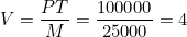
Each rupee therefore changes hands four times a year. As a check, $MV = 25000 \times 4 = 100000$ , which equals $PT$ .

Now suppose the money supply doubles to Rs. 50,000 while velocity remains at 4 and the number of T-shirts sold remains at 100. The equation becomes $50000 \times 4 = P \times 100$ , which gives $P = 2000$ . The same 100 T-shirts now sell for twice the price. Money doubled, prices doubled, and real output did not change.

Situation	M (Rs.)	V	T	P (Rs.)
Initial	25,000	4	100	1,000
After money supply doubles	50,000	4	100	2,000

The result depends entirely on the assumption that V and T did not change. If velocity had halved, because people chose to hold on to their cash, the price level would not have risen at all. If the economy had produced twice as many T-shirts, the price would also have stayed the same. A second example makes the same point. Suppose 60 loaves of bread are sold in a year at Rs. 50 each, so that $PT = 50 \times 60 = 3000$ , and the money supply is Rs. 1,000. Velocity must be $\dfrac{3000}{1000} = 3$ , so each rupee changes hands three times a year.

From Identity to Theory

It is important not to confuse the identity with the theory. The equation $MV = PT$ holds whatever happens, because velocity is, in effect, defined as the number that makes it hold. A theory, by contrast, makes a claim that could be wrong.

The quantity theory becomes a theory when we add the assumption that V and T are stable, determined by forces such as payment habits, institutions and the economy’s productive capacity rather than by the quantity of money.

With that assumption, the identity becomes a causal statement: the money supply determines the price level. Stated compactly, the quantity theory is the equation of exchange plus the assumption that velocity and the volume of transactions are constant.

Fisher’s Transactions Approach

Irving Fisher’s version of the theory is known as the transactions approach, because it focuses on the flow of payments made for transactions during a year. In its simplest form it is the equation $MV = PT$ presented above, and it is often called the Fisher equation. Fisher also wrote a fuller version that recognises that, even in 1911, a large share of payments was made by cheque rather than in cash:

$MV + M'V' = PT$

Here M is the quantity of currency and V its velocity, while $M'$ is the quantity of bank deposits and $V'$ their velocity.

The Determinants of the Price Level

Fisher argued that the price level is determined by three factors.

The first is the volume of trade, which depends on the supply of goods and services to be exchanged. In the long run, he reasoned, the quantity of goods and services produced is determined by the available resources, and since those resources are fully employed, the volume of transactions is fixed.
The second factor is the quantity of money, which is set by monetary authorities outside the model.
The third is the velocity of money, which depends on spending habits, on how frequently wages and other factor payments are made, and on the banking and credit system. These institutional features change only slowly, so velocity can be treated as constant, at least over the short run.

Why Prices Are Proportional to Money

When V and T are held constant, the Fisher equation can be solved for the price level:

$P = \dfrac{V}{T} M$

If we plot the price level against the money supply, the result is a straight line through the origin whose slope is $\dfrac{V}{T}$ . Because the line passes through the origin, any proportional change in M brings the same proportional change in P: a 10% increase in the money supply raises the price level by 10%, and a doubling of the money supply doubles the price level. A change in velocity or in the volume of transactions would change the slope of the line, and the proportionality would then hold only around the new line.

From Transactions to Income

The transactions approach has a practical weakness. The number of transactions is very difficult to measure, because it should include every exchange of goods and services in the economy, including intermediate goods, second-hand goods and purchases of financial assets. National accounts do not record these.

To overcome this difficulty, economists replace the number of transactions T with the economy’s total output Y, which is measured in the national accounts. If P now denotes the price of one unit of output, then $PY$ is the value of total output, which is nominal GDP, and the quantity equation becomes

$MV = PY$

Income Velocity

In this form the velocity of money is called the income velocity of money. It measures the number of times a unit of currency enters someone’s income in a year, or, equivalently, the number of times it is used to buy current output only. Solving the equation for V gives

$V = \dfrac{PY}{M}$

The earlier example of an economy with nominal GDP of Rs. 400 billion and a money supply of Rs. 100 billion, which gave $V = 4$ , was therefore a calculation of income velocity.

Transaction velocity and income velocity are different concepts. Transaction velocity, $\dfrac{PT}{M}$ , counts every exchange, whereas income velocity, $\dfrac{PY}{M}$ , counts only transactions in final output. Because the total value of all transactions is larger than the value of final output, transaction velocity is larger than income velocity for the same stock of money. The practical advantage of income velocity is that it can be computed from published data, since both nominal GDP and the money supply are reported by statistical agencies.

A Theory of Nominal GDP

Once the equation is written in terms of income, the quantity theory takes a particularly simple form. If velocity is held constant, we can write

$M\bar{V} = PY$

where the bar indicates that V is fixed. The equation says that the money supply determines the nominal value of the economy’s output. With velocity given, an economy with more money will have a larger nominal GDP, and an economy with less money a smaller one. The remaining question is how a given nominal GDP divides between prices and real output, and the answer to that question depends on whether we are interested in the price level, in inflation or in the demand for money.

The Quantity Theory as a Theory of the Price Level

To explain the overall level of prices, the quantity theory combines three building blocks. First, the factors of production and the production function determine the economy’s level of real output Y. Second, the supply of money M determines the nominal value of output $PY$ through the quantity equation.

Third, the price level P is simply the ratio of the nominal value of output to the level of real output. In short, the productive capability of the economy determines real GDP, the quantity of money determines nominal GDP, and the GDP deflator is the ratio of nominal GDP to real GDP. Rearranging the quantity equation shows this directly:

$P = \dfrac{M \times V}{Y}$

Because the factors of production and the production function are fixed in the relevant period, real GDP is fixed, and a change in the money supply leads to a proportionate change in nominal GDP and hence in the price level. The quantity theory therefore implies that the price level is proportional to the money supply.

A numerical illustration shows how the formula behaves. Suppose velocity is 4 and real output is 1,000 units, and let the money supply be Rs. 250, giving a price level index of $\dfrac{250 \times 4}{1000} = 1.0$ . If the money supply doubles to Rs. 500, the price level rises to $\dfrac{500 \times 4}{1000} = 2.0$ , and if it triples to Rs. 750, the price level rises to 3.0.

The same formula shows the role of output. If the money supply doubles to Rs. 500 but real output grows by 25% to 1,250 units, the price level rises only to $\dfrac{500 \times 4}{1250} = 1.6$ . More goods chasing the same amount of money mean smaller price increases, which is why economic growth is, other things equal, disinflationary.

Consider one more example with different numbers. Suppose real output is 2,000 units, velocity is 5 and the money supply is Rs. 800. Then 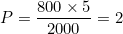$P = \dfrac{800 \times 5}{2000} = 2$ . If the money supply rises by 50% to Rs. 1,200, the price level becomes $\dfrac{1200 \times 5}{2000} = 3$ , an increase of exactly 50%, equal to the increase in the money supply.

The Quantity Theory as a Theory of Inflation

Inflation is the percentage change in the price level, and therefore a theory of the price level is also a theory of the inflation rate. To derive it, we write the quantity equation in percentage-change form:

$\%\Delta M + \%\Delta V = \%\Delta P + \%\Delta Y$

This follows from the fact that the growth rate of a product is approximately the sum of the growth rates of its components. A formal justification takes the natural logarithm of both sides of $MV = PY$ , which gives $\ln M + \ln V = \ln P + \ln Y$ , and then differentiates with respect to time. Percentage changes are close to logarithmic changes when they are small.

Each term in the equation has a straightforward interpretation. The percentage change in the money supply, $\%\Delta M$ , is determined by the central bank. Velocity is assumed to be stable, so $\%\Delta V = 0$ . The percentage change in real GDP, $\%\Delta Y$ , reflects growth in the factors of production and in technology, and it is determined by real rather than monetary forces. The percentage change in the price level, $\%\Delta P$ , is the inflation rate, which is the variable to be explained. Solving for inflation gives

$\%\Delta P = \%\Delta M + \%\Delta V - \%\Delta Y$

When velocity is constant, inflation equals the rate of money growth minus the rate of real output growth. In the simplest version of the theory, where output growth is treated as negligible, the inflation rate equals the rate of growth of the money supply. For example, if money grows by 10% a year, real output grows by 3% and velocity is constant, inflation is $10 + 0 - 3 = 7\%$ .

If velocity were to rise by 1% as well, inflation would be 8%, which shows why a stable velocity matters for the theory. A central bank that wished to achieve zero inflation in this economy would allow the money supply to grow by only 3%, matching the growth of output.

The policy implication is among the most important in macroeconomics. Because the central bank controls the money supply, the quantity theory implies that it has ultimate control over the rate of inflation. If the central bank keeps the money supply stable, the price level will be stable. If it expands the money supply rapidly, the price level will rise rapidly.

Empirical Evidence: Money Growth and Inflation

Milton Friedman summarised this view in a famous remark: “Inflation is always and everywhere a monetary phenomenon.” Friedman, who won the Nobel Prize in economics in 1976, and his collaborator Anna Schwartz documented the sources and effects of changes in the quantity of money over the past century in their monetary history of the United States. Their data, and later data of the same kind, provide two kinds of evidence.

The first is historical. If the average rate of money growth and the average rate of inflation in the United States are plotted for each decade since the 1870s, as in the macroeconomics textbook of N. Gregory Mankiw, the points lie along a rising line. Decades with high money growth, such as the 1970s, tend to have high inflation, while decades with low money growth, such as the 1930s, tend to have low inflation.

The second is international. When the average rate of inflation and the average rate of money growth are plotted for 165 countries and the euro area for the period 1999 to 2007, the same pattern appears. Countries with high money growth, such as Turkey and Belarus, tend to have high inflation, while countries with low money growth, such as Singapore and Switzerland, tend to have low inflation.

An important caution accompanies both results. If we looked at monthly data on money growth and inflation, rather than data averaged over many years, we would not see as close a connection between the two variables. The quantity theory of inflation works best in the long run, not in the short run, because in the short run velocity and real output fluctuate in ways that obscure the underlying relationship.

Hyperinflation

The clearest confirmations of the theory come from hyperinflations, episodes in which prices rise at extraordinary rates. In Germany in 1923, the price level rose roughly a trillion-fold between 1914 and 1923 as the government financed its spending by printing money. In Hungary in 1946, prices at the peak of the episode doubled in less than a day, the most severe inflation on record. In Zimbabwe in 2008, monthly inflation was estimated at tens of billions of percent. These figures are widely cited estimates and should be read as orders of magnitude. Each episode followed large government deficits financed by the creation of money.

Hyperinflations also illustrate the limits of the assumption that velocity is constant. When prices are rising by the day, holding money is extremely costly, because it loses value every hour. People therefore spend money as soon as they receive it, and velocity rises sharply. This increase in velocity pushes prices up even faster than money growth alone would, which is why prices in hyperinflations often outrun the money supply.

The Quantity Theory as a Theory of Money Demand: The Cambridge Approach

The quantity equation can also be interpreted as a theory of the demand for money. This interpretation, known as the Cambridge cash balance approach, is associated with Alfred Marshall and Arthur Cecil Pigou. Where Fisher treated money chiefly as a medium of exchange and focused on the flow of transactions, the Cambridge economists treated money as something that people choose to hold, and they asked how much money households and firms wish to keep in the form of cash balances.

Real Money Balances

The central concept of this approach is real money balances. The quantity of money M is measured in rupees, but what people care about is the amount of goods and services that money can buy. Real money balances, $\dfrac{M}{P}$ , measure the purchasing power of the stock of money: they tell us the quantity of goods and services that the money supply can buy. If the money supply is Rs. 10,000 and the price level index is 2, real balances equal 5,000 units of goods. If the price level doubles to 4 with the money supply unchanged, real balances fall to 2,500 units. Inflation thus erodes the real value of money holdings.

The Money Demand Function

A money demand function describes how much money people wish to hold. According to the Cambridge approach, the demand for real money balances is proportional to real income:

$\left(\dfrac{M}{P}\right)^d = kY$

In this equation k is a constant that measures the proportion of real income that people wish to hold as money. The reasoning is intuitive: people with higher incomes make more and larger transactions and therefore need to hold more money in order to make them. If k is 0.25 and real income is 1,000 units, people want to hold real balances equal to 250 units.

From Money Demand to the Quantity Equation

The connection between the money demand function and the quantity equation is obtained by equating the demand for real money balances with the supply of real money balances, $\dfrac{M}{P}$ . This gives

$\dfrac{M}{P} = kY$

Multiplying both sides by the price level and rearranging yields

$M \times \dfrac{1}{k} = PY$

If we define velocity as $V = \dfrac{1}{k}$ , this becomes

$MV = PY$

which is exactly the quantity equation in its income form. The demand for money and the velocity of money are therefore two sides of the same coin. If people wish to hold a large amount of money relative to their income, which means that k is large, then money circulates slowly and velocity is low. If they hold only a small amount of money, which means that k is small, then money circulates quickly and velocity is high.

k	$V = \dfrac{1}{k}$	Money holdings equal
1/2	2	Six months of income
1/4	4	Three months of income
1/8	8	One and a half months of income
1/12	12	One month of income

The T-shirt economy discussed earlier had a velocity of 4, which corresponds to $k = \dfrac{1}{4}$ : the people in that economy hold three months’ worth of income in the form of money.

Fisher and Cambridge Compared

The two approaches reach the same equation by different routes, and the difference in emphasis has had lasting consequences. Fisher’s analysis centres on the flow of transactions and treats velocity as a feature of the economy’s payment institutions, such as how frequently wages are paid and how developed the banking system is. The Cambridge analysis centres on the stock of money that individuals choose to hold and treats k as the outcome of individual decisions.

Feature	Fisher	Cambridge
Starting point	Flow of transactions	Demand to hold money
Key parameter	V, determined by institutions	k, determined by individual choice
Equation	$MV = PT$	$M = kPY$

Because k is the result of choices, it can be made to depend on variables such as interest rates and expected inflation, which opens the way to a richer theory of money demand. This is the form in which the quantity theory entered modern monetary economics, in Keynes’s theory of liquidity preference and in Friedman’s 1956 restatement of the quantity theory as a theory of the demand for money.

Criticisms and the Modern Status of the Theory

The quantity theory has been criticised on several grounds, and a balanced assessment must take them seriously.

The most fundamental criticism concerns the stability of velocity. Keynesian economists have long argued that velocity is not a constant but a volatile variable that depends on spending habits and on the interest rate, so that changes in the money supply may be offset by changes in velocity. The experience of many countries supports this view. Financial innovation, including credit cards, electronic payments, mobile money and new kinds of deposit accounts, has changed the amount of money that people hold relative to their income, so that k and V drift over time, sometimes unpredictably.

A second criticism concerns the time horizon. The proportionality of prices to money is a long-run proposition, and the theory is much less reliable over short periods. Month-to-month and year-to-year changes in inflation are influenced by supply shocks, exchange rates, expectations and many other factors that the simple theory ignores.

A third concerns monetary policy in practice. Because of the instability of velocity, many central banks abandoned money growth targets in favour of targeting interest rates or the inflation rate directly. In that sense the quantity theory is less often used today as a day-to-day guide to policy.

Nevertheless, the core insight of the theory has survived. The long-run association between money growth and inflation, documented in the historical and international evidence discussed above, is one of the most robust relationships in macroeconomics. Sustained high inflation has almost never occurred without sustained rapid money growth. What the evidence rejects is the assumption of a constant velocity over short horizons, not the proposition that, in the long run, a central bank that creates money too quickly will produce inflation.

Concluding Remarks

The quantity theory of money begins with an identity, the equation of exchange, and becomes a theory by adding the assumption that velocity and real output are determined independently of the quantity of money. From that assumption follow three closely related results.

The price level is proportional to the money supply; the rate of inflation equals the rate of money growth less the rate of real output growth; and the demand for real money balances is a stable fraction of real income. Fisher’s transactions approach and the Cambridge cash balance approach arrive at the same equation from different starting points, one emphasising how money circulates and the other how much people choose to hold.

The theory’s greatest strength is its long-run empirical record, and its greatest weakness is the assumption of a stable velocity in the short run. Students should therefore treat it as a foundation, a first and indispensable account of the relationship between money and prices, on which more complete theories of money, interest rates and inflation are built.

Glossary of Key Terms

Money supply: the stock of money available in the economy at a point in time.
Liquidity: the ease and quickness with which an asset can be exchanged for goods and services.
Velocity of money: the average number of times per year a unit of currency is used to buy goods and services.
Transaction velocity: velocity measured against the total value of all transactions, $V = \dfrac{PT}{M}$ .
Income velocity: velocity measured against nominal GDP, $V = \dfrac{PY}{M}$ .
Nominal GDP: the value of final output at current prices, $PY$ .
Real GDP: the quantity of final output, valued at constant prices, $Y$ .
GDP deflator: the ratio of nominal GDP to real GDP, used as the measure of the price level.
Equation of exchange: the identity $MV = PT$ , or $MV = PY$ , stating that money spent equals money received.
Real money balances: the purchasing power of the stock of money, $\dfrac{M}{P}$ .
Money demand function: the relationship $\left(\dfrac{M}{P}\right)^d = kY$ between desired real balances and real income.

Review Questions and Practice Problems

The following questions are designed to test understanding of the concepts developed in this article.

What is the quantity theory of money, and what two assumptions are needed to move from the equation of exchange to the theory?
What is the equation of exchange, and why is it an identity rather than a theory?
Differentiate transaction velocity from income velocity. Which is larger for a given money supply, and why?
What are real money balances, and how are they affected by inflation?
What is the money demand function, and how is the parameter k related to the velocity of money?
Nominal GDP is Rs. 500 billion and the money supply is Rs. 125 billion. Calculate income velocity and the value of k.
Nominal GDP rises from Rs. 400 billion to Rs. 600 billion while the money supply stays at Rs. 100 billion. By how much does income velocity change?
Real output is 2,000 units, velocity is 5 and the money supply is Rs. 800. Calculate the price level, and then the new price level if the money supply rises by 50%.
The money supply grows by 8% a year, real output grows by 3% and velocity is constant. What is the inflation rate predicted by the quantity theory?
If a government finances a large budget deficit by borrowing from its central bank, what does the quantity theory predict for inflation? What might weaken that prediction in the short run?
Why might monthly data show a weaker relationship between money growth and inflation than data averaged over decades?

For readers who wish to check their work on the numerical problems: the answers to questions 6 to 9 are, respectively, $V = 4$ and $k = 0.25$ ; an increase in velocity from 4 to 6; a price level of 2 rising to 3; and inflation of 5%.

References and Further Reading

Mankiw, N. G. Macroeconomics, chapter on money and inflation.
Fisher, I. (1911). The Purchasing Power of Money.
Friedman, M. (1956). “The Quantity Theory of Money: A Restatement”, in Studies in the Quantity Theory of Money.
Friedman, M. and Schwartz, A. J. (1963). A Monetary History of the United States, 1867 to 1960.
Hume, D. (1752). “Of Money”, in Political Discourses.
Pigou, A. C. (1917). “The Value of Money”, Quarterly Journal of Economics.
Wicksell, K. (1898). Interest and Prices.
Keynes, J. M. (1936). The General Theory of Employment, Interest and Money.

This article is part of the Intermediate Macroeconomics series on Minhaj Metrix Hub. Questions and comments from students and visitors are welcome below.

Share this article

About the author

Muhammad Minhaj Akhtar

Muhammad Minhaj Akhtar is a Lecturer in Economics at Government Graduate College Jauharabad, Pakistan. He holds an M.Phil. in Economics from Quaid-i-Azam University, Islamabad, and an MSc in Economics from the University of Sargodha, where he earned a Silver Medal. His academic passion lies in Econometrics, with a strong focus on applying empirical methods to real-world economic issues. Through MinhajMetrixHub, he shares learning resources, research guidance, and practical econometric insights for students and researchers.

The LM Curve: Liquidity Preference, Money Market Equilibrium, and Its Derivation

Macroeconomics studies how an entire economy behaves by looking at

September 13, 2026 No Comments

Macroeconomics

The IS Curve Explained: Derivation, Slope, and Shift Factors

Macroeconomics studies how an entire economy behaves — how total

September 4, 2026 No Comments

Macroeconomics

Keynesian Cross Model: Equilibrium of National Income Explained

Why does an economy sometimes get stuck producing less than

August 30, 2026 No Comments

Macroeconomics

Intertemporal Consumption Choice: Fisher’s Model of Consumption and Saving

Intertemporal Consumption Choice Fisher’s Model of Consumption and Saving Suppose

August 11, 2026 No Comments

Macroeconomics

Life Cycle Hypothesis of Consumption: 3 Stages of Life Explained

The Life Cycle Hypothesis of Consumption: How Modigliani and Ando

August 10, 2026 No Comments