The LM Curve: Liquidity Preference, Money Market Equilibrium, and Its Derivation

Macroeconomics studies how an entire economy behaves by looking at the interaction of several broad markets at the same time. One of the most important tools economists use for this purpose is the IS-LM model, developed by John Richard Hicks in his 1937 paper “Mr Keynes and the Classics”.

This model explains how the goods market and the money market jointly determine the equilibrium interest rate and the level of national income in the short run.

In our last post, we built the IS curve, which traces combinations of income and the interest rate that keep the goods market in balance. This article focuses on one half of that model, the LM curve, and builds it up step by step, from the basic idea of liquidity preference to a full mathematical and graphical derivation, along with a numerical example.

The Three Markets in Macroeconomics

Before studying the LM curve, it is useful to know where the money market fits into the wider economy. Macroeconomic analysis is usually organised around three major markets.

The Goods Market

The goods market (also called the product market) is where final goods and services are bought and sold. Equilibrium in this market occurs when the total output produced in the economy equals the total planned spending on that output (consumption, investment, government spending, and net exports). The relationship between the interest rate and the level of income that keeps the goods market in equilibrium is summarised by the IS curve.

The Money Market

The money market is where the demand for money and the supply of money interact to determine the equilibrium interest rate. It does not refer to a physical marketplace; rather, it is the conceptual market in which households and firms decide how much of their wealth to hold as money (a liquid, non-interest-earning asset) versus interest-bearing assets such as bonds. The relationship between the interest rate and income that keeps the money market in equilibrium is summarised by the LM curve, which is the subject of this article.

The Labour Market

The labour market is where households supply labour and firms demand labour in exchange for wages. Equilibrium in the labour market, together with the level of output determined in the goods market, helps explain the level of employment and unemployment in the economy.

The IS curve represents equilibrium in the goods market, and the LM curve represents equilibrium in the money market. Together, the IS and LM curves determine the short-run equilibrium interest rate and income level, which in turn interact with the labour market to determine employment.

Demand and Supply of Real Money Balances

Economists analyse the money market in terms of real money balances rather than nominal money, because what matters to people is the purchasing power of the money they hold, not just its face value. Real money balances are written as $M/P$ , where $M$ is the nominal money stock and $P$ is the price level.

Supply of real money balances: The nominal money supply $M$ is set by the central bank (in Pakistan, the State Bank of Pakistan). Since the price level $P$ is fixed in the short run and $M$ is fixed by policy, the supply of real money balances $M/P$ is also fixed at a point in time. On a graph with the interest rate on the vertical axis, the real money supply curve is therefore drawn as a vertical line.

Demand for real money balances: The demand for real money balances, denoted $M^d/P$ , is the quantity of real purchasing power that households and firms wish to hold as money rather than as interest-bearing assets. This demand is negatively related to the interest rate (a higher interest rate raises the opportunity cost of holding non-interest-bearing money) and positively related to real income (higher income means more transactions and therefore a greater need for money). On the same graph, the money demand curve slopes downward.

Money market equilibrium occurs where the demand for real money balances equals the supply of real money balances, and this intersection determines the equilibrium interest rate for a given level of income.

Liquidity Preference and the Three Motives for Holding Money

The theory behind the demand for money was presented by John Maynard Keynes in his 1936 book “The General Theory of Employment, Interest and Money”. Keynes used the term ‘liquidity preference’ to describe people’s demand for money; since money is the most liquid of all assets, it can be spent immediately at no conversion cost. Keynes argued that people are willing to give up this liquidity and hold interest-bearing assets such as bonds instead, only if they are compensated through interest. In this sense, the interest rate is the “price” of giving up liquidity. Keynes identified three motives that lead people to hold money.

Transactions Motive

People hold money to make regular, day-to-day payments, such as buying food, paying rent, and covering transport costs. This transactional demand for money is directly related to the volume of transactions people carry out and therefore rises with the level of income.

Precautionary Motive

People also hold money as a buffer against unforeseen events, such as sudden illness, accidents, or emergency expenses. Like the transactions motive, precautionary demand for money is positively related to income, since higher-income individuals typically want a larger cash buffer.

Speculative Motive

Speculation refers to buying and selling assets such as bonds and securities in the hope of profiting from short-term price movements. Bond prices and interest rates move in opposite directions. When the interest rate is low (bond prices are high), people expect rates to rise in the future (and bond prices to fall), so they prefer to hold money rather than bonds. When the interest rate is high (bond prices are low), holding cash becomes costly, so people prefer to hold bonds and hold less money. This is the motive that creates the negative relationship between money demand and the interest rate.

These together imply that money demand is positively related to income Y (transactions and precautionary motives) and negatively related to the interest rate (speculative motive).

Money Market Equilibrium and the Adjustment Process

Money market equilibrium is reached at the interest rate where the quantity of real money balances supplied equals the quantity demanded.

Money supply (Ms) is fixed by the central bank at a point in time, so it is drawn as a vertical line. Money demand (Md) slopes downward: people want to hold less money and more bonds as the interest rate rises.

Point E is equilibrium: the interest rate r* at which the quantity of money demanded exactly equals the fixed quantity supplied for the given income level Y. But how does the market actually reach this point if the interest rate starts away from equilibrium?

Figure 1: Money Market Equilibrium & Adjustment Process

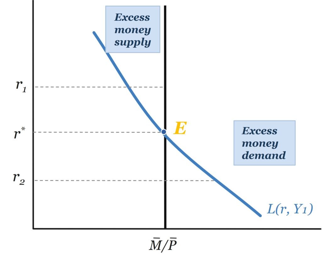
If the interest rate is above equilibrium (r*), the quantity of real money balances supplied exceeds the quantity demanded. People holding this excess money supply use it to buy interest-bearing assets such as bonds. This raises the demand for bonds, and bond issuers and banks respond by lowering the interest rate they offer. As the interest rate falls, the quantity of money demanded rises until equilibrium is restored.

If the interest rate is below equilibrium (r*), the quantity of money demanded exceeds the quantity supplied. People try to obtain more money by selling bonds or making bank withdrawals. To attract funds that are now scarcer, banks and bond issuers raise the interest rate they offer. As the interest rate rises, the quantity of money demanded falls until equilibrium is restored.

This adjustment process shows that the interest rate is not fixed by decree; it is pulled toward equilibrium by the buying and selling of bonds whenever the money market is out of balance.

Measures of Money Supply in Pakistan

Central banks, including the State Bank of Pakistan (SBP), track several measures of the money supply, ranging from the narrowest and most liquid to progressively broader aggregates. These aggregates are commonly labeled M0 through M3.

Measure	Also Known As	Composition
M0	Reserve money / monetary base	Currency in circulation, plus commercial banks’ deposits (reserves) with the SBP, plus other deposits held with the SBP. This is the most liquid measure and the base on which the rest of the money supply is built.
M1	Narrow money	Currency in circulation held by the public, plus demand deposits (current accounts) with scheduled banks, plus other deposits with the SBP. M1 includes only assets that can be used directly and immediately as a medium of exchange.
M2	Broad money	M1, plus time deposits and resident foreign currency deposits held with scheduled banks. M2 is the aggregate the SBP monitors most closely as its primary indicator of monetary conditions, since it also captures close assets, though slightly less liquid, money substitutes.
M3	Broader money	A wider aggregate that extends M2 (or, in some classifications, M1) by including other relatively less liquid financial assets, such as additional deposits with non-bank financial institutions. M3 is used mainly for detailed academic and statistical analysis rather than routine monetary policy targeting.

In practice, the SBP publishes and targets broad money (M2) as its key monetary aggregate, while M0 (reserve money) is what the central bank most directly controls through its open market operations.

What Is the LM Curve?

The LM curve stands for liquidity preference and money supply. It shows all the combinations of the interest rate and the level of income at which the money market is in equilibrium.

The LM curve is derived directly from Keynes’s liquidity preference theory: at each level of income, the equilibrium interest rate is determined by the intersection of the demand for and supply of real money balances.

Since money demand is negatively related to the interest rate and positively related to income, while the money supply is fixed by the central bank, an increase in income raises money demand at every interest rate. Because the money supply does not change, the interest rate must rise to bring money demand back down to the fixed money supply. This is why higher income is associated with a higher equilibrium interest rate, and it is the reason the LM curve slopes upward.

Step-by-Step Mathematical Derivation of the LM Curve

The graphical logic above can be expressed precisely using algebra. The derivation below follows five steps.

Step 1: Money Market Equilibrium

Equilibrium in the money market requires that the real money supply equal the real money demand:

$\frac{M}{P} = \frac{M^{d}}{P}$

Here, $M$ is the nominal money supply set by the central bank, $P$ is the price level, so $M/P$ is the real value of money balances, and $M^{d}$ is nominal money demand.

Step 2: The Liquidity Preference Function

Money demand can be written as a general function, $L(\cdot)$ , of the nominal interest rate and income:

$\frac{M}{P} = L(r + \pi^{e},\, Y)$

By the Fisher equation, the nominal interest rate is $i = r + \pi^{e}$ , where $r$ is the real interest rate and $\pi^{e}$ is expected inflation. Money demand rises with income $Y$ through the transactions and precautionary motives, and falls as the nominal interest rate rises through the speculative motive.

Step 3: A Linear Money Demand Function

To derive a precise equation for the LM curve, the liquidity preference function $L(\cdot)$ is written as a straight line:

$\frac{M}{P} = c_{0} + c_{1}Y - c_{2}(r + \pi^{e})$

Here, $c_{0}$ is autonomous money demand, the baseline level of money demand that does not depend on $Y$ or $r$ ; $c_{1}$ measures the sensitivity of money demand to income, with $c_{1} > 0$ ; and $c_{2}$ measures the sensitivity of money demand to the interest rate, with $c_{2} > 0$ .

Step 4: Isolating the Interest Rate

To solve for the interest rate, the interest-sensitive term is first moved to the left-hand side of the equation:

$\frac{M}{P} + c_{2}(r + \pi^{e}) = c_{0} + c_{1}Y$

Then $M/P$ is moved to the right-hand side, isolating the interest-rate term:

$c_{2}(r + \pi^{e}) = c_{0} + c_{1}Y - \frac{M}{P}$

Step 5: Solving for r — The LM Equation

Dividing both sides by $c_{2}$ gives:

$r + \pi^{e} = \frac{c_{0}}{c_{2}} + \left(\frac{c_{1}}{c_{2}}\right)Y - \frac{1}{c_{2}}\left(\frac{M}{P}\right)$

Subtracting $\pi^{e}$ from both sides isolates the real interest rate, $r$ :

$r = \left[\frac{c_{0}}{c_{2}} - \pi^{e}\right] + \left(\frac{c_{1}}{c_{2}}\right)Y - \frac{1}{c_{2}}\left(\frac{M}{P}\right)$

This equation links the real interest rate $r$ and income $Y$ for a given money supply and price level, it is the LM curve. Writing 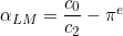$\alpha_{LM} = \dfrac{c_{0}}{c_{2}} - \pi^{e}$ as the intercept and $\beta_{LM} = \dfrac{c_{1}}{c_{2}}$ as the slope, the LM curve can be stated in general form as:

$r_{LM} = \alpha_{LM} - \frac{1}{c_{2}}\left(\frac{M}{P}\right) + \beta_{LM}Y$

For comparison, the IS curve in the same general notation is $r_{IS} = \alpha_{IS} - \beta_{IS}Y$ : the LM curve slopes upward in $(Y, r)$ space and shifts with $M$ and $P$ , while the IS curve slopes downward and shifts with fiscal policy variables such as government spending $G$ and taxes $T$ .

Graphical Derivation of the LM Curve

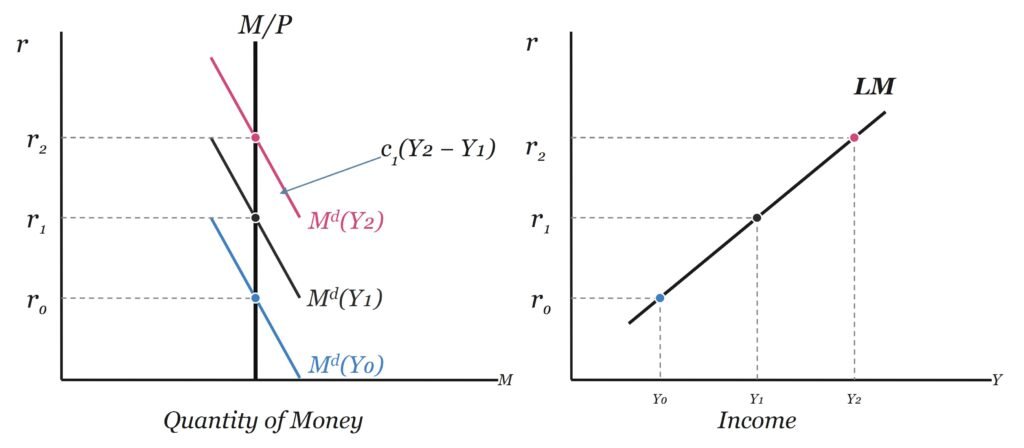
The mathematics above can also be shown graphically using two side-by-side diagrams: the money market on the left and the LM curve on the right.

Figure 2: Derivation of LM Curve from Liquidity Preference Theory

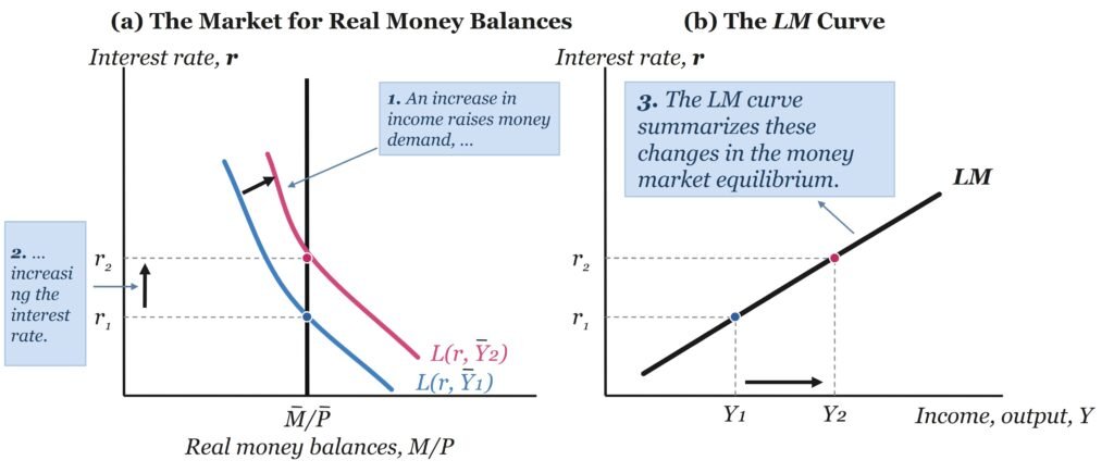
In the money market diagram, the real money supply $M^{s} = M/P$ is drawn as a vertical line, since it is fixed by the central bank at a point in time. The money demand curve $L(r, Y)$ slopes downward against the interest rate. At income level $Y_{1}$ , money demand is $L(r, Y_{1})$ , and the equilibrium interest rate is $r_{1}$ , the point where this demand curve crosses the fixed money supply line.

Now suppose income rises from $Y_{1}$ to $Y_{2}$ . Because money demand increases with income, the entire money demand curve shifts to the right, to $L(r, Y_{2})$ . At the original interest rate $r_{1}$ , the quantity of money demanded now exceeds the fixed money supply. This excess demand for money pushes the interest rate up until it reaches a new, higher equilibrium, $r_{2}$ .

Each pair of income and its corresponding equilibrium interest rate, $(Y_{1}, r_{1})$ and $(Y_{2}, r_{2})$ , can then be plotted on a second diagram with income on the horizontal axis and the interest rate on the vertical axis. Connecting all such equilibrium pairs traces out the LM curve.

Because a higher level of income always requires a higher interest rate to keep the money market in equilibrium, given a fixed money supply, the LM curve slopes upward.

Slope of the LM Curve and the Factors That Affect It

From the general LM equation, the slope of the LM curve with respect to income is:

$\beta_{LM} = \frac{c_{1}}{c_{2}}$

Since both $c_{1}$ and $c_{2}$ are positive, this slope is always positive, confirming that the LM curve slopes upward. How steep or flat the curve is depends on two elasticities.

Elasticity of Money Demand	When High	When Low
Interest elasticity of money demand ( $c_2$ )	LM curve is flatter	LM curve is steeper
Income elasticity of money demand ( $c_1$ )	LM curve is steeper	LM curve is flatter

Figure 3: High Interest Elasticity of Money Demand

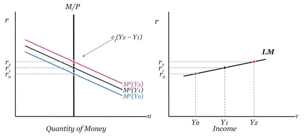
Figure 4: Low Interest Elasticity of Money Demand

The intuition is straightforward. If money demand is highly sensitive to the interest rate ( $c_{2}$ is large), only a small change in the interest rate is needed to absorb the extra money demand created by a rise in income, so the LM curve is relatively flat.

If money demand barely responds to the interest rate ( $c_{2}$ is small), a much larger change in the interest rate is required, making the LM curve steep. Similarly, if money demand is highly sensitive to income ( $c_{1}$ is large), a given rise in income creates a large increase in money demand, which requires a bigger rise in the interest rate to restore equilibrium, again making the LM curve steeper.

Shift Factors of the LM Curve

A change in income causes a movement along a given LM curve. A shift of the entire LM curve, however, is caused by a change in one of the variables that were held fixed while drawing it. There are three such shift factors.

Factor	Increase	Decrease
Money supply, $M$	LM curve shifts downward / to the right	LM curve shifts upward / to the left
Price level, $P$	Real balances $M/P$ fall, LM curve shifts upward / to the left	Real balances $M/P$ rise, LM curve shifts downward / to the right
Autonomous money demand, $c_{0}$	LM curve shifts upward / to the left	LM curve shifts downward / to the right

Changes in Money Supply

The LM curve shows a given level of the money supply. If the central bank reduces the money supply, the real money supply curve shifts left, raising the equilibrium interest rate at every level of income and shifting the entire LM curve upward. An increase in the money supply has the opposite effect, shifting the LM curve downward.

Changes in the Price Level

Because it is the real money supply, $M/P$ , that matters for equilibrium, a rise in the price level reduces real balances even if the nominal money supply $M$ is unchanged. This has the same effect as a fall in the money supply: it shifts the LM curve upward. A fall in the price level shifts the LM curve downward.

Shifts in Money Demand

A shift in the money demand function means that the amount of money demanded changes at every given level of the interest rate and income, what Keynes called a shift in liquidity preference. This can happen, for example, because of a loss of confidence in bonds, which increases the demand for money and shifts the LM curve upward, or because of new payment technology that reduces the need to hold cash, which shifts the LM curve downward.

A Numerical Example

The abstract equation from Section 7 becomes clearer with actual numbers. Suppose the linear money demand function is:

$\frac{M^{d}}{P} = 500 + 0.1\,Y - 1000\,(r + \pi^{e})$

so that $c_{0} = 500$ , $c_{1} = 0.1$ , and $c_{2} = 1000$ . Suppose further that the economy is given the following values:

$\frac{M}{P} = 400, \qquad Y = 1000, \qquad \pi^{e} = 0.02$

Substituting these values into the LM equation derived in Step 5:

$r = \left[\frac{500}{1000} - 0.02\right] + \frac{0.1}{1000}(1000) - \frac{1}{1000}(400)$

$r = 0.48 + 0.10 - 0.40$

$r = 0.18 \ \text{or} \ 18\%$

So, when income is 1,000, the money market clears at a real interest rate of 18 percent. Now consider what happens if income rises to $Y = 1200$ , holding $M/P$ and $\pi^{e}$ unchanged:

$r = \left[\frac{500}{1000} - 0.02\right] + \frac{0.1}{1000}(1200) - \frac{1}{1000}(400) = 0.48 + 0.12 - 0.40 = 0.20 \ \text{or} \ 20\%$

The two equilibrium pairs, $(Y = 1000,\ r = 18\%)$ and $(Y = 1200,\ r = 20\%)$ , both lie on the same LM curve. As income rose by 200, the equilibrium interest rate rose by 2 percentage points, exactly matching the slope $\beta_{LM} = c_{1}/c_{2} = 0.1/1000 = 0.0001$ , since $0.0001 \times 200 = 0.02$ . This confirms, with real numbers, that the LM curve is upward sloping.

Key Takeaways

Macroeconomics is organized around the goods market, the money market, and the labor market; the LM curve summarizes equilibrium in the money market.
Money demand depends positively on income (transactions and precautionary motives) and negatively on the interest rate (speculative motive), while the real money supply is fixed by the central bank at a point in time.
Money market equilibrium occurs where real money demand equals real money supply; deviations from equilibrium are corrected through the buying and selling of bonds, which pushes the interest rate back to its equilibrium level.
The State Bank of Pakistan tracks several money supply measures, from the narrowest (M0, reserve money) to progressively broader aggregates (M1, M2, and M3), with M2 serving as its main policy-relevant aggregate.
The LM curve, $r = \alpha_{LM} - \dfrac{1}{c_{2}}\left(\dfrac{M}{P}\right) + \beta_{LM}Y$ , traces every combination of income and the interest rate that clears the money market, and it always slopes upward.
The slope of the LM curve, $\beta_{LM} = c_{1}/c_{2}$ , is steeper when money demand is more sensitive to income or less sensitive to the interest rate.
The LM curve shifts, rather than merely moving along itself, when the money supply, the price level, or autonomous money demand changes.

Share this article

About the author

Muhammad Minhaj Akhtar

Muhammad Minhaj Akhtar is a Lecturer in Economics at Government Graduate College Jauharabad, Pakistan. He holds an M.Phil. in Economics from Quaid-i-Azam University, Islamabad, and an MSc in Economics from the University of Sargodha, where he earned a Silver Medal. His academic passion lies in Econometrics, with a strong focus on applying empirical methods to real-world economic issues. Through MinhajMetrixHub, he shares learning resources, research guidance, and practical econometric insights for students and researchers.